Week 3.5 - Deriving 4th order approximation of a 2nd order derivative using Taylor Table method

Aim: To derive a fourth-order approximation of second-order derivative using the Taylor table method and compare the different schemes.

Objective: 1. To derive central skewed-right and skewed-left differencing schemes

2. Compare the absolute error with the analytical derivative using function `f(x) = exp(x)*cos(x)`

Theory:

Usually, in CFD problems, we decide the order of accuracy that we need, according to it we decide the scheme. For deriving different schemes of different orders we use the Taylor table method. The stencil we use may be symmetric or asymmetric.

For a given order of derivative, the order of approximation depends on the total number of nodes used in the stencil.

For the symmetric stencil, order of approximation = number of nodes in stencil - order of derivative +1

For the Asymmetric stencil, order of approximation = number of nodes in stencil - order of derivative

Central difference fourth-order approximation

`(partial^2u)/(partialx^2) = (af(i-2)+bf(i-1)+cf(i)+df(i+1)+ef(i+2))/(Deltax^2)`

The numbers of nodes that should be used from the expression, which is mentioned above. As the central differencing scheme is symmetrical the number of nodes we have to consider is 5 (4+2-1).

Here f is the hypothesis function and its coefficients are what we are going to determine.

write the hypothesis function in the left column of the Taylor table and Taylor series terms in the top row.

Taylor table for central difference

	`f(i)`	`Deltaxf^1(i)`	`Deltax^2f^2(i)`	`Deltax^3f^3(i)`	`Deltax^4f^4(i)`	`Deltax^5f^5(i)`
`af(i-2)`	a	-2a	2a	-8a/6	16a/24	-32a/120
`bf(i-1)`	b	-b	b/2	-b/6	b/24	-b/120
`cf(i)`	c	0	0	0	0	0
`df(i+1)`	d	d	d/2	d/6	d/24	d/120
`ef(i+2)`	e	2e	2e	8e/6	16e/24	32e/120
	0	0	1	0	0

we obtain the algebraic equations from the summation of columns.

then there will be 5 equations with 5 unknowns.

these equations can be solved by arranging them in the matrix form as Ax = B

by using matrix inversion the solution matrix is found.

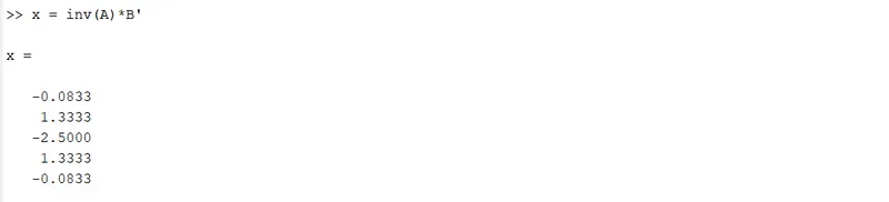
we use these values for completing the expression for the central differencing scheme.

Similarly, the same method is applied for skewed schemes. The only difference would be the number of nodes considered in the stencil.

Skewed right-sided differencing scheme

In this scheme, the nodes are considered only from the right side. Hence it is asymmetric. The number of nodes to be considered is 6 (4+2).

`(partial^2u)/(partialx^2) = (af(i)+bf(i+1)+cf(i+2)+df(i+3)+ef(i+4)+gf(i+5))/(Deltax^2)`

Taylor table for skewed right

	`f(i)`	`Deltaxf^1(i)`	`Deltax^2f^2(i)`	`Deltax^3f^3(i)`	`Deltax^4f^4(i)`	`Deltax^5f^5(i)`
`af(i)`	a	0	0	0	0	0
`bf(i+1)`	b	b	b/2	b/6	b/24	b/120
`cf(i+2)`	c	2c	2c	8c/6	16c/24	32c/120
`df(i+3)`	d	3d	9d/2	27d/6	81d/24	243d/120
`ef(i+4)`	e	4e	16e/2	64e/6	256e/24	1024e/120
`gf(i+5)`	g	5g	25g/2	125g/6	625g/24	3125g/120
	0	0	1	0	0	0

summation of the columns give 6 equations with six unknowns. Separate variable and coefficients and for a matric equation in the form Ax = B

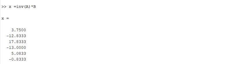
Skewed left-sided differencing

Similar to the right-sided scheme on the number of nodes but we consider left-sided nodes

	`f(i)`	`Deltaxf^1(i)`	`Deltax^2f^2(i)`	`Deltax^3f^3(i)`	`Deltax^4f^4(i)`	`Deltax^5f^5(i)`
`af(i)`	a	0	0	0	0	0
`bf(i+1)`	b	-b	b/2	-b/6	b/24	-b/120
`cf(i+2)`	c	-2c	2c	-8c/6	16c/24	-32c/120
`df(i+3)`	d	-3d	9d/2	-27d/6	81d/24	-243d/120
`ef(i+4)`	e	-4e	16e/2	-64e/6	256e/24	-1024e/120
`gf(i+5)`	g	-5g	25g/2	-125g/6	625g/24	-3125g/120
	0	0	1	0	0	0

and coefficients are

Code

main code :

clear 
close all
clc

%program for fourth order approximation of second order derivative
%Analytical derivative of exp(x)*cos(x) is -2*exp(x)*sin(x)

x = pi/3;
%grid size
dx = linspace(pi/4,pi/400,200);

%preallocating for changing size for every loop
central_differencing_approximation = ones(1,length(dx));
skewed_right_sided = ones(1,length(dx));
skewed_left_sided = ones(1,length(dx));

for i = 1:length(dx)
    central_differencing_approximation(i) = fourth_order_central_approx(x,dx(i));
    skewed_right_sided(i) = fourth_order_right_skewed(x,dx(i));
    skewed_left_sided(i) = fourth_order_left_skewed(x,dx(i));
end

%plotting the results
figure(1)
loglog(dx,central_differencing_approximation,'b','linewidth',2)
hold on
loglog(dx,skewed_right_sided,'k','linewidth',2)
hold on
loglog(dx,skewed_left_sided,'r','linewidth',2)
xlabel('range of dx')
ylabel('absolute error')
grid on
title('consistency of different schemes')
legend('central differencing','right differencing','left differencing','Location','northwest')

Function for the central differencing scheme

function error_central = fourth_order_central_approx(x,dx)
    A = [1 1 1 1 1;-2 -1 0 1 2;2 1/2 0 1/2 2;-8/6 -1/6 0 1/6 8/6;16/24 1/24 0 1/24 16/24];
    B = [0;0;1;0;0];
    x_c = A\B;
    Analytical_derivative = -2*exp(x)*sin(x);
    %numerical derivative by central differencing approximation
    Numerical_derivative = ((x_c(1)*f_x(x-2.*dx))+(x_c(2)*f_x(x-dx))+(x_c(3)*f_x(x))+(x_c(4)*f_x(x+dx))+(x_c(5)*f_x(x+2.*dx)))./dx.^2;
    error_central = abs(Analytical_derivative - Numerical_derivative);
end

Function for the skewed-right

function error_right = fourth_order_right_skewed(x,dx)
    A = [1 1 1 1 1 1;0 1 2 3 4 5;0 1/2 2 9/2 8 25/2;0 1/6 8/6 27/6 64/6 125/6;0 1/24 16/24 81/24 256/24 625/24;0 1/120 32/120 243/120 1024/120 3125/120];
    B = [0; 0; 1; 0; 0; 0];
    x_r = A\B;
    Analytical_derivative = -2*exp(x)*sin(x);
    %numerical derivative by central differencing approximation
    Numerical_derivative = (((x_r(1))*((exp(x))*(cos(x))))+((x_r(2))*((exp(x+dx))*(cos(x+dx))))+((x_r(3))*((exp(x+(2.*dx)))*(cos(x+(2.*dx)))))+((x_r(4))*((exp(x+(3*dx)))*(cos(x+(3.*dx)))))+((x_r(5))*((exp(x+(4.*dx)))*(cos(x+(4*dx)))))+((x_r(6))*((exp(x+(5.*dx)))*(cos(x+(5.*dx))))))./(dx.^2);
    error_right = abs(Analytical_derivative - Numerical_derivative);
end

Function for the skewed left

function error_left = fourth_order_left_skewed(x,dx)
    A = [1 1 1 1 1 1;0 1 2 3 4 5;0 1/2 2 9/2 8 25/2;0 1/6 8/6 27/6 64/6 125/6;0 1/24 16/24 81/24 256/24 625/24;0 1/120 32/120 243/120 1024/120 3125/120];
    B = [0; 0; 1; 0; 0; 0];
    x_l = A\B;
    Analytical_derivative = -2*exp(x)*sin(x);
    %numerical derivative by central differencing approximation
    Numerical_derivative = (((x_l(6))*((exp(x-(5.*dx)))*(cos(x-(5.*dx)))))+((x_l(5))*((exp(x-(4.*dx)))*(cos(x-(4.*dx)))))+((x_l(4))*((exp(x-(3.*dx)))*(cos(x-(3.*dx)))))+((x_l(3))*((exp(x-(2.*dx)))*(cos(x-(2.*dx)))))+((x_l(2))*((exp(x-dx))*(cos(x-dx))))+((x_l(1))*((exp(x))*(cos(x)))))./(dx.^2);
    error_left = abs(Analytical_derivative - Numerical_derivative);
end

In the main code first, we define the value of x and grid size.

We define the schemes by using functions and we preallocate the functions as these are changing size in the loop.

then we call each function in for loop and calculate values for each and every grid size.

loglog plot is used for the study of errors as it gives a good picture of variation in the error.

Plots

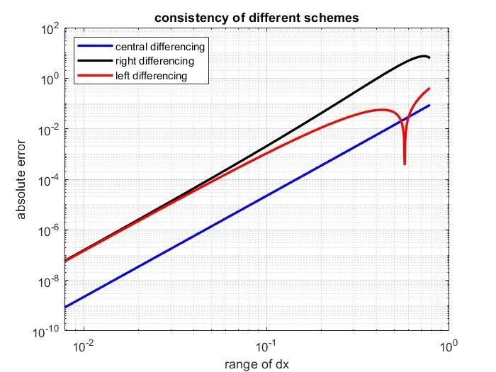
As we can see that central differencing scheme has least error compared to other two schemes.

Skewed schemes are useful when we are trying to solve governing equations at boundaries. There won't be enough nodes on any one of the sides then the central differencing scheme may not be helpful as it is symmetric and requires same number of nodes on both sides. In this case skewed schemes are helpful.

Problems encountered during MATLAB programming : While using the coefficients i have manually entered the values in the equation that has caused the error. It is called round off errors as the decimals we enter are not completely equal to the obtained values. Rather I accessed the solution matrix of coefficients with indexing.