Week 3 - Solving second order ODEs

Aim: To simulate the motion of a simple pendulum by solving the ordinary differential equation of motion of the pendulum.

Governing equation: `(d^2θ)/(dt^2)+(b/m)(dθ)/dt+g/Lsinθ=0`

this is the ode for the motion of a simple pendulum with a damping effect.

Procedure:

• First, define the function to solve the ode which is a second-order differential equation. This can be done by splitting the ode into two parts by assuming variables. arrange them in the form of a vector.
• Also, define the inputs in the function.
• In the main program define 't', a time span. Here we have to simulate for 20 seconds.
• [t y] = ode45('odefun',t,y0), where y0 is the initial conditions. For a second-order, we need to have two conditions. I have taken the theta as y for simplicity.
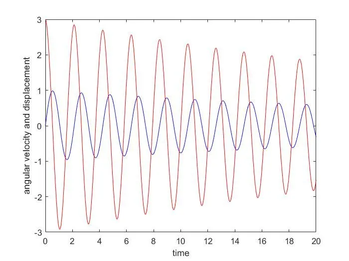
• after solving the ode plot the results for angular velocity and displacement with respect to time.
• As for the animation for each time step, the graph is plotted on the same figure, and lines and markers are used to show the pendulum by calculating the positions from the displacement values.
• Finally, all the plots are compiled into a video.

Code:

close all
clear all
clc

%solving some ode

t = linspace(0,20,500); %starting time and ending time
y0 =[0 3]; %initial condition

[t y] = ode45('odefun',t,y0);

%plotting of angular velocity and displacement 
plot(t,y(:,1),'color','b')
hold on
plot(t,y(:,2),'color','r')
ylabel('angular velocity and displacement')
xlabel('time')
hold off

% Pendulum Animation
ct=1;
for i=1:length(y(:,1))
x0 = 0;
y0 = 0;
x1 =1*sin(y(i,1));
y1 =-(1*cos(y(i,1)));
figure(2)
plot([-1,1],[0,0],'linewidth',3,'color','b');
hold on 
plot([x0 x1], [y0 y1],'linewidth',3,'color','k');
hold off 
hold on
plot(x1,y1,'o','markersize',20,'markerfacecolor','r','markeredgecolor','r');
hold off
title('Simulation of a Damped Pendulum Motion');
grid on 
axis([-1.5 1.5 -1.5 .5]);

M(ct)=getframe(gcf);
ct = ct + 1;
end

% Video of the animation
movie(M)
video=VideoWriter('Pendulum.avi','Uncompressed AVI');
open(video)
writeVideo(video,M)
close(video)

Function code

function [ydot] = odefun(t,y)
l =1;
m = 1;
b=0.05;
g =9.81;

  ydot = zeros(2,1);
  ydot(1)=y(2);
  ydot(2) = -(b/m) * y(2)-(g/l) * sin(y(1));
end

Results:

plot:

Animation:

In the plot, The red plot is for Velocity vs time and the other one displacement and time. The plots vary with the damping factor.