Week 7 - Simulation of a 1D Super-sonic nozzle flow simulation using Macormack Method

Aim :- To simulate the isentropic flow through a quasi 1D subsonic-supersonic nozzle and derive conservation and non-conservation forms of the governing equations and sovle them using the MacCormack's technique. Determine the steady-state temperature distribution for the flow-field variables and investigate the difference between the two forms of governing equations by comparing their solutions.

Show plots for -

1. Steady-state distribution of primitive variables inside the nozzle
2. Time-wise variation of the primitive variables
3. Variation of Mass flow rate distribution inside the nozzle at different time steps during the time-marching process
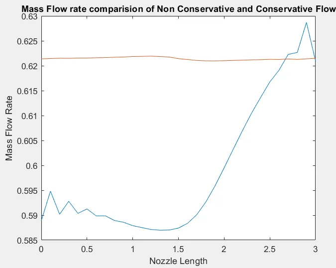
4. Comparison of Normalized mass flow rate distributions of both forms

Introduction :-

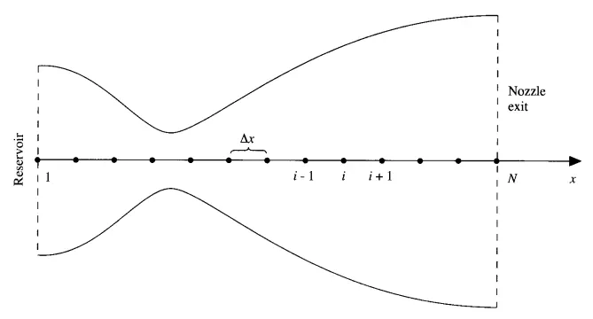
We consider the steady and isentropic flow through a convergent-divergent nozzle. In Subsonic inlet we assume that cross sectional area of the resorvoir is large so that the velocity is considerd very small. As we move along the flow the f;ow expands Insentropically to supersonic speeds at the nozzle exit. The inlets and outlets are denoted in the figure below.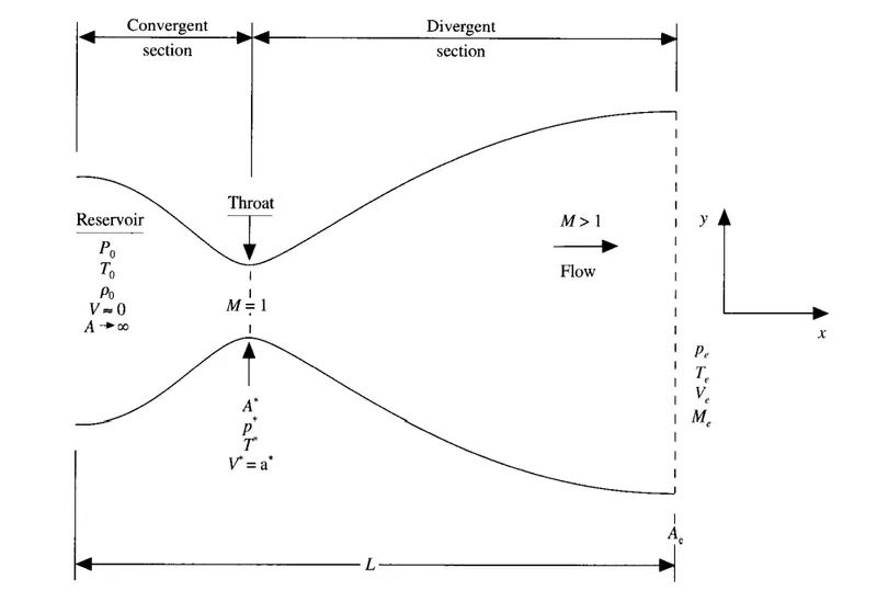

The force that is excerted on the gas to accelarate through the nozzle. The force is supplied by the pressure ratio across the nozzle `[(P)underset(o)() ]/ [(P)underset(e)() ]`.

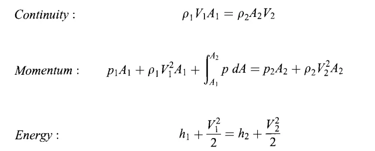
Area of the nozzle changes as the function along the direction of the nozzle. As it is in 2D we assume that flow properties are uniform across a given section. This type of flow is defined as quasi 1D flow.

Analytical Solution :-

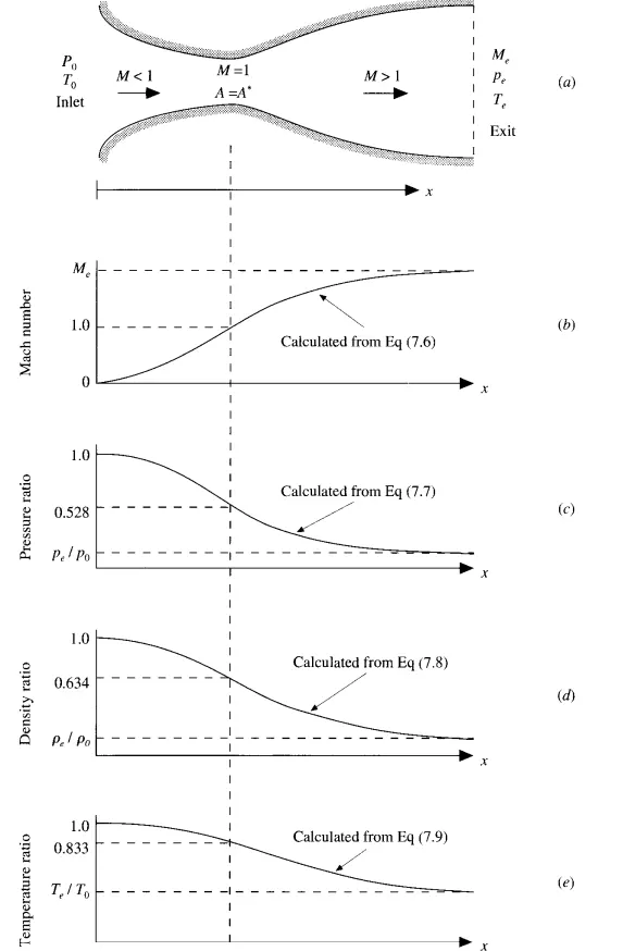
We solve the equations analatically. From the flow through the nozzle we find that the Mach number variation through the nozzle is covered by the area ratio `[A/A^**]`.

`gamma =` ratio of specific heat `[cunderset(p)() ]/[cunderset(v)() ]` { For air it is 1.4}

Area ratio is f(x).

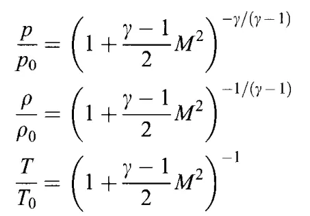
If the area relation is f(x) then we can say that the variation of pressure, density and temperature as the function of Mach Number. And hence the function of `[A/A^**]` and f(x) is given by the equation

Governing Equations for Non Conservative Form :-

These are formulated in Partial Differential form which are sutable for time marching solutions for Quasi 1D Flow.

For the Nozzle flow the flow field variables are frequently expressed in terms of the Non-Dimentional variables. Non-Dimentional variables vary between 0 & 1.

Reservoir Temperature `T' = T/[Tunderset(0)()]`

Reservoir Density `rho' = rho / [rhounderset(0)()]`

Dimensionless Length `x' = x/L`

Dimensionless Velocity `V' = [V] /[aunderset(0)()]`

Dimensionless Time `t' = t/[L/[aunderset(0)()]`

Dimensionless Area `A' = A/A^**`

By implementing the finite difference MacCormack's technique for a numarical solution of Governing Equation we divide the x-axis along the nozzle into a number of grid points. MacCormack's technique is a Predictor Corrector method which is a second order diff in both space and time.

Predictor step :-

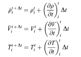
We use Forward differencing scheme for spacial derivatives for predictor step & we are going to calculate the solution variant for which we obtain an intermediate solution. These are the discretised governing equation we use for the predictor step.

Intermediate Solution

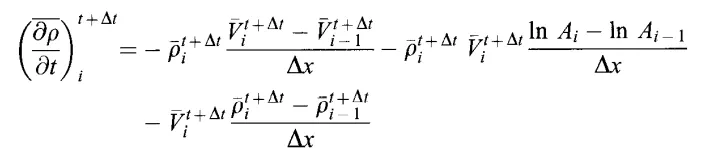
Corrector step :-

We First obtained a correctod value of the time derivative at time `t + Deltat` . This corrected values are obtained by substituting the predictor values of `rho`,`V`& `t` into the right side of the equation & replace the space derivative with this backword differencing

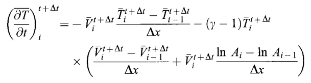
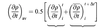
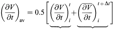
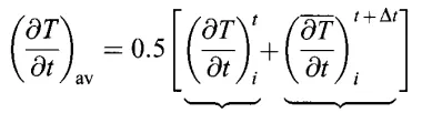
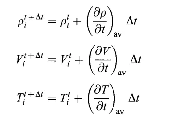
Final Solution :- We are going to caculate the average values of the derivatives which are obtained from the arethamatic mean of the Predictor and Corrector step this allowes us to obtain the final value of density ,velocity & temperatue at time `t + Deltat` .

Governing Equation for Conservative Form :-

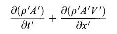
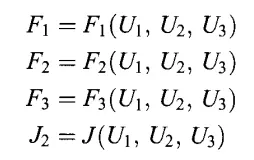
In this the Partial Differentiation is similar to Non-Conservative Form. We express this equation into a generic form by defining the elements of Solution Vector `U` , Flux Vector `F` & the Source Vector `J` .

Continuity

Momentum

Energy

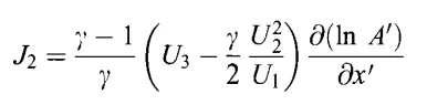
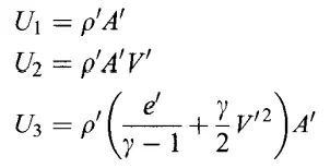
The first terms inside this derivatives of governing equation are taken as solution vectors `Uunderset(1)(), Uunderset(2)() & Uunderset(3)()` .The second term inside the derivatives of this equationare taken as Flux Vectors `Funderset(1)() , Funderset(2)() & Funderset(3)()`. We have a source term `Junderset(2)()` in momentum equation.

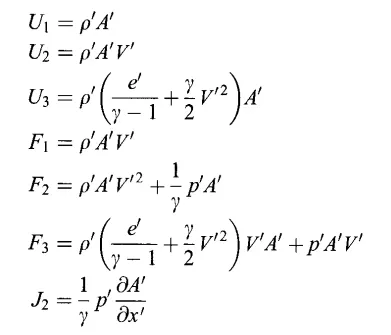
In conservative form all this values represent the continuity, momentum & energy.

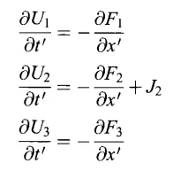
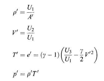
We have setup a numarical solution for `Uunderset(1)() , Uunderset(2)() & Uunderset(3)()` at each time step.We then decode this elements of solution vector `U` to obtain the premitive variables at each time step.

Before moving into MacCormack's technique the premitive variables are used to construct `Funderset(1)() ,Funderset(2)() & Funderset(3)()`. Some numarical difficulties might aries for that reason the governing equations are written in pure form that is in terms of `Uunderset(1)() , Uunderset(2)() & Uunderset(3)()` only.

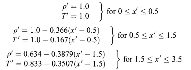
Initial Conditions

Solution Variable Initialization

Pritictor setp :-

The Flux terms are initialized before starting of the predictor step in the MacCormack's technique. Now we employ the predictor step in MacCormack's technique using the forword differencing scheme spacial derivative to calculate the flux term we obtain the intermediate solutions by using the predictor values and old values of solution vectors. The Premitive variables such as `V , T & P` are computed from the obtained updated values of `Uunderset(1)() , Uunderset(2)() & Uunderset(3)()` from the equtaions.

Initialization of Flux

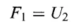
`Funderset(1)() = Uunderset(2)()`

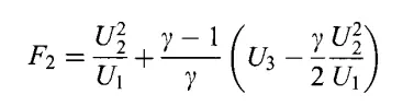
`Funderset(2)() = (U^2underset(1)() )/(Uunderset(1)()) + (gamma - 1)/gamma (Uunderset(3)() - gamma/2 (U^2underset(1)())/[Uunderset(1)()])`

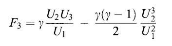
`Funderset(3)() = gamma [Uunderset(2)() Uunderset(3)()]/[Uunderset(1)()] - [gamma(gamma-1)]/2 [U^3underset(2)()]/[U^2underset(1)()]`

`J^t underset(1)()(i) = (1/gamma).rho(i).T(i).([A(i+1)-A(i)]/dx)`

Corrector Step :-

Here we obtain the corrected values of time derivatives at time `t + Deltat` by substituting the predictor values of `Funderset(1)(), Funderset(2)() & Funderset(3)()` in the right side of the equation & also replacing the spacial derivatives with the Backword differences. We calculate time derivative of the solution vectors `Uunderset(1)(), Uunderset(2)() & Uunderset(3)()` from the corrector derivatives of `Funderset(1)(), Funderset(2)() & Funderset(3)()` . We then proced to calculate the average of the derivatives `Uunderset(1)(), Uunderset(2)() & Uunderset(3)()` from the predicted and corrected time derivatives.

`([delUunderset(1)()]/[delt])underset(avg)() = 0.5 [ ([overline[delUunderset(1)()]]/[delt])^tunderset(i)() + ([delUunderset(1)()]/[delt])^[t+Deltat]underset(i)()]`

`([delUunderset(2)()]/[delt])underset(avg)() = 0.5 [ ([overline[delUunderset(2)()]]/[delt])^tunderset(i)() + ([delUunderset(2)()]/[delt])^[t+Deltat]underset(i)()]`

`([delUunderset(3)()]/[delt])underset(avg)() = 0.5 [ ([overline[delUunderset(3)()]]/[delt])^tunderset(i)() + ([delUunderset(3)()]/[delt])^[t+Deltat]underset(i)()]`

Final Solution :-

It is obtained from the calculated average derivatives and the old values of solution vectors.

`Uunderset(1)()^[t+Deltat](i) = Uunderset(1)()^t(i) + ([delUunderset(1)()]/[delt])underset(avg)() . Deltat`

`Uunderset(2)()^[t+Deltat](i) = Uunderset(2)()^t(i) + ([delUunderset(2)()]/[delt])underset(avg)() . Deltat`

`Uunderset(3)()^[t+Deltat](i) = Uunderset(3)()^t(i) + ([delUunderset(3)()]/[delt])underset(avg)() . Deltat`

`rho' = [Uunderset(1)()] /[A']`

`V' = [Uunderset(2)()]/[Uunderset(1)()]`

`T' = e' = (gamma-1)([Uunderset(3)()]/[Uunderset(1)()]-gamma/2V'^2)`

`p' = rho'T'`

Code :-

clear all
close all
clc

% Non Conservative
% inputs
L = 3 ;
n = 31 ;
x = linspace(0,L,n) ;
dx = x(2)-x(1) ;

% gamma
G = 1.4 ;

% Calculate initial profiles
rho_Nc = 1-0.3146*x ;
t_Nc = 1-0.2314*x ;      % Time
v_Nc = (0.1 + 1.09*x).*t_Nc.^0.5 ;

% Area
a = 1 + 2.2*(x-1.5).^2 ;

% Time steps
nt = 1400 ;
dt = 0.0201 ;

% Outer time loop
for k = 1:nt
    
    %Predictor method
    rho_old = rho_Nc ;
    v_old = v_Nc ;
    t_old = t_Nc ;
    
    for j = 2:n-1 
    
    dvdx = (v_Nc(j+1) - v_Nc(j))/dx ;       
    drhodx = (rho_Nc(j+1) - rho_Nc(j))/dx ; 
    dtdx = (t_Nc(j+1) - t_Nc(j))/dx ;       
    dlogadx = (log(a(j+1)) - log(a(j)))/dx ;
    
    % Continuty equation
    drhodt_p(j) = -rho_Nc(j)*dvdx - rho_Nc(j)*v_Nc(j)*dlogadx - v_Nc(j)*drhodx ;
    % Momentum equation
    dvdt_p(j) = -v_Nc(j)*dvdx - (1/G)*(dtdx + (t_Nc(j)/rho_Nc(j))*drhodx) ;
    % Energy equation
    dtdt_p(j) = -v_Nc(j)*dtdx - (G-1)*t_Nc(j)*(dvdx + v_Nc(j)*dlogadx) ;
    
    
    % Solution update
    rho_Nc(j) = rho_Nc(j) + drhodt_p(j)*dt ;
    v_Nc(j) = v_Nc(j) + dvdt_p(j)*dt ;
    t_Nc(j) = t_Nc(j) + dtdt_p(j)*dt ;
    end

% Corrector method

    for j = 2:n-1 
    
    dvdx = (v_Nc(j) - v_Nc(j-1))/dx ;       
    drhodx = (rho_Nc(j) - rho_Nc(j-1))/dx ; 
    dtdx = (t_Nc(j) - t_Nc(j-1))/dx ;       
    dlogadx = (log(a(j)) - log(a(j-1)))/dx ;
    
    % Continuty equation
    drhodt_c(j) = -rho_Nc(j)*dvdx - rho_Nc(j)*v_Nc(j)*dlogadx - v_Nc(j)*drhodx ;
    % Momentum equation
    dvdt_c(j) = -v_Nc(j)*dvdx - (1/G)*(dtdx + (t_Nc(j)/rho_Nc(j))*drhodx) ;
    % Energy equation
    dtdt_c(j) = -v_Nc(j)*dtdx - (G-1)*t_Nc(j)*(dvdx + v_Nc(j)*dlogadx) ;
    
    % Solution update
    rho_Nc(j) = rho_Nc(j) + drhodt_c(j)*dt ;
    v_Nc(j) = v_Nc(j) + dvdt_c(j)*dt ;
    t_Nc(j) = t_Nc(j) + dtdt_c(j)*dt ;
    end
    
% Compute the average time derivative
drhodt = 0.5*(drhodt_p + drhodt_c) ;
dvdt = 0.5*(dvdt_p + dvdt_c) ;
dtdt = 0.5*(dtdt_p + dtdt_c) ;

% Final solution update
for i = 2:n-1
%     rho_old = rho ;
%     v_old = v ;
%     t_old = t ;
    
    rho_Nc(i) = rho_old(i) + drhodt(i)*dt ;
    v_Nc(i) = v_old(i) + dvdt(i)*dt ;
    t_Nc(i) = t_old(i) + dtdt(i)*dt ;
    
end

% Apply the boundry conditions
% Inlet 
v_Nc(1) = 2*v_Nc(2) - v_Nc(3) ;
% Outlet
rho_Nc(n) = 2*rho_Nc(n-1) - rho_Nc(n-2) ;
v_Nc(n) = 2*v_Nc(n-1) - v_Nc(n-2) ;
t_Nc(n) = 2*t_Nc(n-1) - t_Nc(n-2);
 
% calculation
m_Nc = rho_Nc.*1.*v_Nc.*1.*a ;       % Mass flow rate
mach_Nc = v_Nc./((t_Nc).^0.5) ;      % Mach number
p_Nc = rho_Nc.*t_Nc ;                % Pressure


% throt conditions
throat = find(a==1) ;
rho_t(k) = rho_Nc(throat) ;        % Density at throat
t_t(k) = t_Nc(throat) ;            % Temparature at throat
p_t(k) = p_Nc(throat) ;            % Preassure at throat
mach_t(k) = mach_Nc(throat) ;      % Mach number at throat


% Plotting
figure(1)
if k == 0
    plot(x,m_Nc,'black')
    hold on
elseif k == 50
    plot(x,m_Nc,'r')
    hold on
elseif k == 100
    plot(x,m_Nc,'m')
    hold on
elseif k == 150
    plot(x,m_Nc,'b')
    hold on
elseif k == 200
    plot(x,m_Nc,'y')
    hold on
elseif k == 700
    plot(x,m_Nc,'g')
    hold on
end
xlabel('Nondimensional distence through Nozzil') ;
ylabel('Nondimensional Mass Flow') ;
% legend({'50','100','150','200','700'}) ;
title('Mass Flow rate at different Timesteps - Non Conservative') ;

axis([0 3 0 2])




end

figure(2)
% Density
subplot(4,1,1) ;
plot(x,rho_Nc,'r') ;
xlabel('Nozzil Domain') ;
ylabel('Density ratio') ;
legend({'Density'}) ;
title('Variation of Flow along length of the Nozzil - Non Conservative') ;
% Temparature
subplot(4,1,2) ;
plot(x,t_Nc,'b') ;
xlabel('Nozzil Domain') ;
ylabel('Temparature ratio') ;
legend({'Temparature'}) ;
% Pressure
subplot(4,1,3) ;
plot(x,p_Nc,'g') ;
xlabel('Nozzil Domain') ;
ylabel('Pressure ratio') ;
legend({'Pressure'}) ;
% Mach Number
subplot(4,1,4) ;
plot(x,mach_Nc,'m') ;
xlabel('Nozzil Domain') ;
ylabel('Mach Number ratio') ;
legend({'Mach Number'}) ;


figure(3) 
% Density
subplot(4,1,1) ;
plot(1:nt,rho_t,'r');
xlabel('Number of Timesteps') ;
ylabel('Density') ;
legend({'Density at throat'}) ;
title('Timestep at throat - Non Conservative') ;
% Temparature
subplot(4,1,2) ;
plot(1:nt,t_t,'b');
xlabel('Number of Timesteps') ;
ylabel('Temparature') ;
legend({'Temparature at throat'}) ;
% Pressure
subplot(4,1,3) ;
plot(1:nt,p_t,'g');
xlabel('Number of Timesteps') ;
ylabel('Pressure') ;
legend({'Pressure at throat'}) ;
% Mach Number
subplot(4,1,4) ;
plot(1:nt,mach_t,'m');
xlabel('Number of Timesteps') ;
ylabel('Mach Number') ;
legend({'Mach Number at throat'}) ;



% Conservative

% inputs
L = 3 ;
n = 31 ;
x = linspace(0,L,n) ;
dx = x(2)-x(1) ;

G = 1.4 ;                   % gamma
a = 1 + 2.2*(x-1.5).^2 ;    % Area

% Initial Conditions
for i = 1:n 
    
    if (x(i)>=0 && x(i)<=0.5)
        rho_C(i) = 1;
        t_C(i) = 1;
    elseif (x(i)>=0.5 && x(i)<=1.5)
        rho_C(i) = 1-0.366*(x(i)-0.5);
        t_C(i) = 1-0.167*(x(i)-0.5);
    elseif (x(i)>=1.5 && x(i)<=3.5)
        rho_C(i) = 0.634-0.3879*(x(i)-1.5);
        t_C(i) = 0.833-0.3507*(x(i)-1.5);
    end
end

c = 0.579 ;                 % constent
v_C = 0.59./(rho_C.*a) ;        % Assuming initial conditions

u1 = rho_C.*a ;
u2 = rho_C.*a.*v_C ;              % u2 = u1*v
H = (t_C/(G-1)) + (G/2)*v_C.^2 ;
u3 = rho_C.*H.*a ;
p_C = rho_C.*t_C ;                  % Pressure



% Time steps
nt = 1400 ;
dt = 0.0267 ;  % min(-(c)*((dx)*u1)/u2) ;


% Outer time loop
for k = 1:nt

    u1_old = u1;
    u2_old = u2;
    u3_old = u3;
    
 % Time steps 
F1 = u2 ;
F2 = ((u2.^2./u1)) + ((G-1)/G)*(u3-(G/2)*(u2.^2./u1)) ;
F3 = (G*(u2.*u3)./u1) - G*((G-1)/2)*(u2.^3/u1.^2) ;
    
     for j = 2:n-1 
    
    %Predictor method
         
    du1dx = (F1(j+1) - F1(j))/dx ;       
    du2dx = (F2(j+1) - F2(j))/dx ; 
    du3dx = (F3(j+1) - F3(j))/dx ;
    dadx = (a(j+1) - a(j))/dx ;
    %J = ((G-1)/G)*(u3-(G/2)*u2.^2./u1)*dlogadx ;
    J = (1/G)*rho_C.*t_C.*dadx;
  
    du1dt_p(j) = -(du1dx) ;
    du2dt_p(j) = -(du2dx) + J(j) ;
    du3dt_p(j) = -(du3dx) ;
    
  %  Dt = 0.0267 ;  % 
    
    % Solution update
    u1(j) = u1(j) + du1dt_p(j)*dt ;
    u2(j) = u2(j) + du2dt_p(j)*dt ;
    u3(j) = u3(j) + du3dt_p(j)*dt ;
    
     end
     
 F1 = u2 ;
 F2 = ((u2.^2./u1)) + ((G-1)/G)*(u3-(G/2)*(u2.^2./u1)) ;
 F3 = (G*(u2.*u3)./u1) - G*((G-1)/2)*(u2.^3/u1.^2) ;
     
   % Corrector method
  
    for j = 2:n-1 
        
    du1dx = (F1(j) - F1(j-1))/dx ;       
    du2dx = (F2(j) - F2(j-1))/dx ; 
    du3dx = (F3(j) - F3(j-1))/dx ;
    dadx = (a(j) - a(j-1))/dx ;
    J = (1/G)*rho_C.*t_C.*dadx;
    
    du1dt_c(j) = -(du1dx) ;
    du2dt_c(j) = -(du2dx) + J(j) ;
    du3dt_c(j) = -(du3dx) ;
    
  %  Dt = 0.0267 ;  % 
    
    % Solution update
    u1(j) = u1(j) + du1dt_c(j)*dt ;
    u2(j) = u2(j) + du2dt_c(j)*dt ;
    u3(j) = u3(j) + du3dt_c(j)*dt ;
    end
    
    % Compute the average time derivative
    du1dt = 0.5*(du1dt_p + du1dt_c) ;
    du2dt = 0.5*(du2dt_p + du2dt_c) ;
    du3dt = 0.5*(du3dt_p + du3dt_c) ;
    
    
  % Final solution update
for i = 2:n-1
    
    u1(i) = u1_old(i) + du1dt(i)*dt ;
    u2(i) = u2_old(i) + du2dt(i)*dt ;
    u3(i) = u3_old(i) + du3dt(i)*dt ;
    
end
        
 % Apply the boundry conditions
 % Inlet
 u1(1) = rho_C(1)*a(1);
 u2(1) = 2*u2(2) - u2(3);
 v_C(1) = u2(1)/u1(1) ;
 u3(1) = u1(1)*((t_C(1)/(G-1))+(G/2)*v_C(1)^2);
 
 % Outlet
 u1(n) = 2*u1(n-1) - u1(n-2);
 u2(n) = 2*u2(n-1) - u2(n-2);
 u3(n) = 2*u3(n-1) - u3(n-2);
 
 % In terms
 rho_C = u1./a ;
 v_C = u2./u1 ;
 t_C = (G-1)*((u3./u1)-((G*v_C.^2)/2)) ;
 
% calculation
m_C = rho_C.*v_C.*a ;             % Mass flow rate
mach_C = v_C./((t_C).^0.5) ;      % Mach number
p_C = rho_C.*t_C ;                % Pressure


% throt conditions
throat = find(a==1) ;
rho_t(k) = rho_C(throat) ;        % Density at throat
t_t(k) = t_C(throat) ;            % Temparature at throat
p_t(k) = p_C(throat) ;            % Preassure at throat
mach_t(k) = mach_C(throat) ;      % Mach number at throat
 

% Plotting
figure(4)
if k == 0
    plot(x,m_C,'black')
    hold on
elseif k == 50
    plot(x,m_C,'r')
    hold on
elseif k == 100
    plot(x,m_C,'m')
    hold on
elseif k == 150
    plot(x,m_C,'b')
    hold on
elseif k == 200
    plot(x,m_C,'y')
    hold on
elseif k == 700
    plot(x,m_C,'g')
    hold on
end
axis([0 3 0 2])
xlabel('Nondimensional distence through Nozzil') ;
ylabel('Nondimensional Mass Flow') ;
% legend({'50','100','150','200','700'}) ;
title('Mass Flow rate at different Timesteps - Conservative') ;

 
end

figure(5)
% Density
subplot(4,1,1) ;
plot(x,rho_C,'r') ;
xlabel('Nozzil Domain') ;
ylabel('Density ratio') ;
legend({'Density'}) ;
title('Variation of Flow along length of the Nozzil - Conservative') ;
% Temparature
subplot(4,1,2) ;
plot(x,t_C,'b') ;
xlabel('Nozzil Domain') ;
ylabel('Temparature ratio') ;
legend({'Temparature'}) ;
% Pressure
subplot(4,1,3) ;
plot(x,p_C,'g') ;
xlabel('Nozzil Domain') ;
ylabel('Pressure ratio') ;
legend({'Pressure'}) ;
% Mach Number
subplot(4,1,4) ;
plot(x,mach_C,'m') ;
xlabel('Nozzil Domain') ;
ylabel('Mach Number ratio') ;
legend({'Mach Number'}) ;


figure(6) 
% Density
subplot(4,1,1) ;
plot(1:nt,rho_t,'r');
xlabel('Number of Timesteps') ;
ylabel('Density') ;
legend({'Density at throat'}) ;
title('Timestep at throat - Conservative') ;
% Temparature
subplot(4,1,2) ;
plot(1:nt,t_t,'b');
xlabel('Number of Timesteps') ;
ylabel('Temparature') ;
legend({'Temparature at throat'}) ;
% Pressure
subplot(4,1,3) ;
plot(1:nt,p_t,'g');
xlabel('Number of Timesteps') ;
ylabel('Pressure') ;
legend({'Pressure at throat'}) ;
% Mach Number
subplot(4,1,4) ;
plot(1:nt,mach_t,'m');
xlabel('Number of Timesteps') ;
ylabel('Mach Number') ;
legend({'Mach Number at throat'}) ;

% Mass Flow rate comparision of Non Conservative and Conservative Flow
figure(7)
plot(x,m_Nc);
hold on
plot(x,m_C) ;
xlabel('Nozzle Length');
ylabel('Mass Flow Rate');
title('Mass Flow rate comparision of Non Conservative and Conservative Flow')

Figure 1

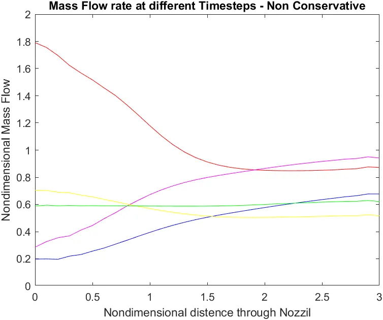
Figure 2

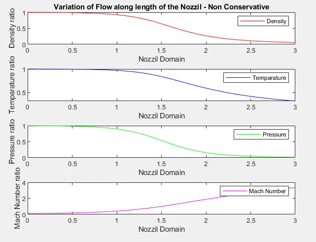
Figure 3

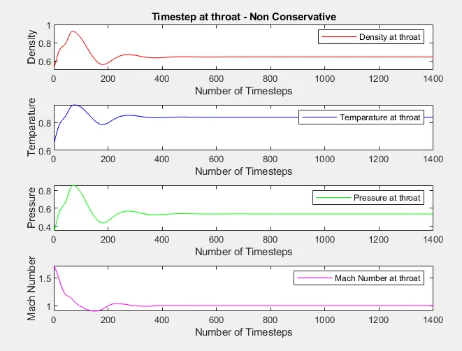
Figure 4

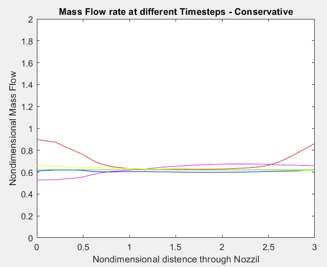
Figure 5

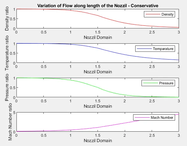
Figure 6

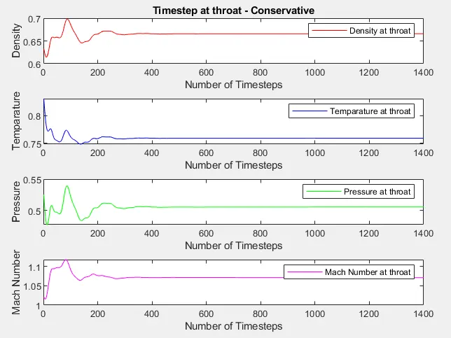
Figure 7

Conclusion :-

Non-Conservative form is more accurate for primitive variables such as Density, Pressure ,Temperature. And Conservative form is closer to accurate for Flux variables such as Mass Flow rate. Non-Conservative Form gives closer results for analytical solutions.