Week 3.5 - Deriving 4th order approximation of a 2nd order derivative using Taylor Table method

1) Derivation of Central difference

Number of nodes in the stencil (N) = The order of accuracy (P) + Order of derivative (Q) - 1

P = 4 ; Q = 2

(-2,-1,0,1,2)

`(del^2f)/(delx^2) = a f(i-2) + b f(i-1) + c f(i) + d f(i+1) + e f(i + 2)`

	f(i)	`f'(i)*dx`	`f''(i)*dx^2`	`f'''(i)*dx^3`	`f''''(i)*dx^4`
a f(i - 2)	a	-2a	4a	-8a/6	16a/24
b f(i - 1)	b	-b	b/2	-b/6	b/24
c f(i)	c	0	0	0	0
d f(i + 1)	d	d	d/2	d/6	d/24
e f(i + 2)	e	2e	4e	8e/6	16e/24
`sum`	0	0	1	0	0

A*X = B

`[[1,1,1,1,1],[-2,-1,0,1,2],[2,1/2,0,1/2,2],[-4/3,-1/6,0,1/6,4/3],[2/3,1/24,0,1/24,2/3]]`*`[[a],[b],[c],[d],[e]]`= `[[0],[0],[1],[0],[0]]`

`f'' = (-1*f[i-2]+16*f[i-1]-30*f[i+0]+16*f[i+1]-1*f[i+2])/(12*h^2)`

2) Derivation of Skewed right-sided difference

Number of nodes in the stencil (N) = The order of accuracy (P) + Order of derivative (Q)

P = 4 ; Q = 2

(0,1,2,3,4,5)

`(del^2f)/(delx^2) = a f(x) + b f(i +1) + c f(i + 2) + d f(i + 3) + e f(i + 4) + f f(i + 5)`

	`f(i)`	`f'(i)*dx`	`f''(i)*dx^2`	`f'''(i)*dx^3`	`f''''(i)*dx^4`	`f'''''(i)*dx^5`
a f(i)	a	0	0	0	0	0
b f(i + 1)	b	b	b/2	b/6	b/24	b/120
c f(i + 2)	c	2c	4c/2	8c/6	16c/24	32c/120
d f(i + 3)	d	3d	9d/2	27d/6	81d/24	243d/120
e f(i + 4)	e	4e	16e/2	64e/6	256e/24	1024e/120
f f(i + 5)	f	5f	25f/2	125f/6	625f/24	3125f/120
`sum`	0	0	1	0	0	0

A*X = B

`[[1,1,1,1,1,1],[0,1,2,3,4,5],[0,1/2,2,9/2,8,25/2],[0,1/6,4/3,9/2,32/3,125/6],[0,1/24,2/3,27/8,32/3,625/24],[0,1/120,4/15,81/40,128/15,625/24]]`*`[[a],[b],[c],[d],[e],[f]]`=`[[0],[0],[1],[0],[0],[0]]`

`f'' = (45*f[i+0]-154*f[i+1]+214*f[i+2]-156*f[i+3]+61*f[i+4]-10*f[i+5])/(12*h^2)`

3) Derivation of Skewed right-sided difference

Number of nodes in the stencil (N) = The order of accuracy (P) + Order of derivative (Q)

P = 4 ; Q = 2

(-5,-4,-3,-2,-1,0)

`(del^2f)/(delx^2) = a f(i - 5) + b f(i - 4) + c f(i - 3) + d f(i - 2) + e f(i -1) + f f(x)`

	`f(i)`	`f'(i)*dx`	`f''(i)*dx^2`	`f'''(i)*dx^3`	`f''''(i)*dx^4`	`f'''''(i)*dx^5`
a f(i - 5)	a	-5a	25a/2	-125a/6	625a/24	-3125a/120
b f(i - 4)	b	-4b	16b/2	-64b/6	256b/24	-1024b/120
c f(i - 3)	c	-3c	9c/2	-27c/6	81c/24	-243c/120
d f(i - 2)	d	-2d	4d/2	-8d/6	16d/24	-32d/120
e f(i - 1)	e	-e	e/2	-e/6	e/24	-e/120
f f(i)	f	0	0	0	0	0
`sum`	0	0	1	0	0	0

A*X = B

`[[1,1,1,1,1,1],[-5,-4,-3,-2,-1,0],[25/2,8,9/2,2,1/2,0],[-125/6,-32/3,-9/2,-4/3,-1/6,0],[625/24,32/3,27/8,2/3,1/24,0],[-625/24,-128/15,-81/40,-4/15,-1/120,0]]`*`[[a],[b],[c],[d],[e],[f]]`=`[[0],[0],[1],[0],[0],[0]]`

`f'' = (-10*f[i-5]+61*f[i-4]-156*f[i-3]+214*f[i-2]-154*f[i-1]+45*f[i+0])/(12*h^2)`

clear all
close all
clc
% analytical function f(x) = exp(x)*cos(x) ;
% analytical derivative 
% f'(x) = exp(x)*(-sin(x)) + exp(x)*cos(x) ;
% f''(x) =  -2*exp(x)*sin(x) ;
x = pi/3 ;
analytical_derivative = (-2*exp(x)*sin(x)) ;


dx = linspace(pi/4000,pi/40,20)  ;


for i=1:length(dx)
    
    X = exp(x)*cos(x) ;
    X_1 = exp(x+(1*dx(i)))*cos(x+(1*dx(i))) ;
    X_11 = exp(x-(1*dx(i)))*cos(x-(1*dx(i))) ;
    X_2 = exp(x+(2*dx(i)))*cos(x+(2*dx(i))) ;
    X_22 = exp(x-(2*dx(i)))*cos(x-(2*dx(i))) ;
    X_3 = exp(x+(3*dx(i)))*cos(x+(3*dx(i))) ;
    X_33 = exp(x-(3*dx(i)))*cos(x-(3*dx(i))) ;
    X_4 = exp(x+(4*dx(i)))*cos(x+(4*dx(i))) ;
    X_44 = exp(x-(4*dx(i)))*cos(x-(4*dx(i))) ;
    X_5 = exp(x+(5*dx(i)))*cos(x+(5*dx(i))) ;
    X_55 = exp(x-(5*dx(i)))*cos(x-(5*dx(i))) ;

    
   % Central difference
   central_differencing = ((-1*X_22)+(16*X_11)-(30*X)+(16*X_1)-(1*X_2))/(12*1*dx(i).^2) ;
   % Skewed right-sided difference
   skewed_right_sided_difference = ((45*X)-(154*X_1)+(214*X_2)-(156*X_3)+(61*X_4)-(10*X_5))/(12*1*dx(i).^2) ;
   % Skewed left-sided difference
   skewed_left_sided_difference =  ((-10*X_55)+(61*X_44)-(156*X_33)+(214*X_22)-(154*X_11)+(45*X))/(12*1*dx(i).^2) ;
   
   error_central_differencing(i) = abs(central_differencing - analytical_derivative) ;
   error_skewed_right_sided_difference(i) = abs(skewed_right_sided_difference - analytical_derivative) ;
   error_skewed_left_sided_difference(i) = abs(skewed_left_sided_difference - analytical_derivative) ;
end

%plot
figure(1);
loglog(dx,error_central_differencing,'g','marker','*')
hold on
loglog(dx,error_skewed_right_sided_difference,'r','marker','^')
hold on
loglog(dx,error_skewed_left_sided_difference,'b','marker','+')
hold off
xlabel('dx')
ylabel('error')
title('4th Order Approximation of a 2nd Order Derivative')
legend('error central differencing','error skewed right-sided difference','error skewed left-sided difference')

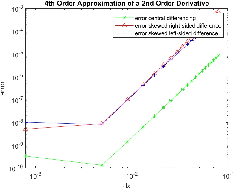
Explanation

Compared to forward diffrencing scheme and backward differencing scheme skewed scheme provides a more accurate result because of getting more available information from many points. It can be used for solving when points available on one side.

Central difference can't be used when there are no left and right points here skewed scheme can be used to follow points in a particular direction.