Simulation of an isentropic flow through a Quasi 1D Super-sonic nozzle using McCormack Method
OBJECTIVE
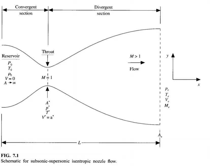
To simulate the isentropic flow through a quasi 1D subsonic-supersonic nozzle using the conservation and non-conservation forms of the governing equations and sovle them using the MacCormack's technique.
- Perform a grid independence test on the solution
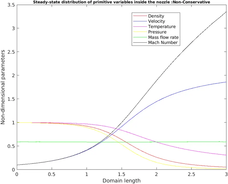
- Plot the steady-state distribution of primitive variables inside the nozzle
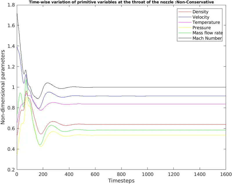
- Plot the time-wise variation of the primitive variables
- Plot the variation of Mass flow rate distribution inside the nozzle at different time steps during the time-marching process
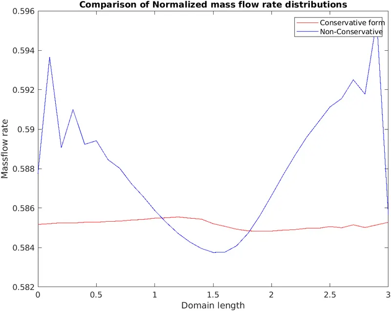
- Comparison of Normalized mass flow rate distributions of both forms
McCORMACK'S TECHNIQUE
Let `f(x)` be the function to be solved. This technique involves 5 steps to be followed in order.
- Initial profile
All the flow field variables are to be determined in this step.
- Predictor step
A predicted derivative is found using the forward differencing scheme.
`((delf)/(delt))_p=(f_(i+1)-f_i)/(Deltax)`
- Solution update
The derivative found in earlier step is added to the old values and updated.
`f_p=f_(old)+((delf)/(delt))_p*dt`
- Corrector step
The updated solution needs to be treated with corrector variable. This corrector variable is found by
`((delf_p)/(delt))_c=(f_i-f_(i-1))/(Deltax)`
- Average time derivative
An average time derivative is found that is to be added to the initial values of f.
`((delf)/(delt))_(avg)=0.5(((delf)/(delt))_p+((delf_p)/(delt))_c)`
- Final solution update
The final solution or the next timestep value for the function would be
`f^(n+1)=f_(old)+((delf)/(delt))_(avg)*dt`
NON-CONSERVATIVE FORM OF GOVERNING EQUATIONS
- Continuity equation: `(delp)/(delt)=-rho(delv)/(delx)-rhov(del(lnA))/(delx)-v(delrho)/(delx)`
- Momentum equation: `(delv)/(delt)=-v(delv)/(delx)-(1/gamma)((delT)/(delx)+T/rho.(delrho)/(delx))`
- Energy equation: `(delT)/(delt)=-v(delT)/(delx)-(gamma-1)T((delv)/(delx)+v(del(lnA))/(dx))`
CONSERVATIVE FORM OF GOVERNING EQUATIONS
- Continuity equation: `(del(rhoA))/(delt)+(del(rhoAv))/(delx)=0`
- Momentum equation: `(del(rhoAv))/(delt)+(del(rhoAv^2))/(delx)=-A(delrho)/(delx)`
- Energy equation: `(del(rhoAv^2/2))/(delt)+(del(rhoAv^3/2))/(delx)=-Av(delrho)/(delx)`
MATLAB CODE
- Main code
% Code for McCormack method of solving Quasi 1D supersonic-subsonic nozzle
% ------------------------------------------------------------------------

 clear all
 close all
 clc

 L=3;                  % Length of nozzle
 n= [31 61 91];        % Number of nodes
 CFL= 0.5;             % Courant number
 nt= 1600;             % Timesteps

 for i= n

     % Calling Non-conservative and Conservative functions respectively
       [rho_NC_t,T_NC_t,p_NC_t,v_NC_t,Mach_NC_t,massflowrate_NC_t,massflowrate_NC]= nonconservative_fun(i,L,CFL,nt);
       [rho_C_t,T_C_t,p_C_t,v_C_t,Mach_C_t,massflowrate_C_t,massflowrate_C]= conservative_fun(i,L,CFL,nt);

       x= linspace(0,L,i);

     if i==31
     % Plotting Time-wise variation of the primitive variables at throat
       figure(5)
       plot(1:nt,rho_NC_t,'r',1:nt,v_NC_t,'b',1:nt,T_NC_t,'m',1:nt,p_NC_t,'y',1:nt,massflowrate_NC_t,'g',1:nt,Mach_NC_t,'k')
       hold on
       ylabel('Non-dimensional parameters')
       xlabel('Timesteps')
       title('Time-wise variation of primitive variables at the throat of the nozzle :Non-Conservative','FontSize',8)
       legend('Density','Velocity','Temperature','Pressure','Mass flow rate','Mach Number')

     % Plotting Time-wise variation of the primitive variables at throat
       figure(6)
       plot(1:nt,rho_C_t,'r',1:nt,v_C_t,'b',1:nt,T_C_t,'m',1:nt,p_C_t,'y',1:nt,massflowrate_C_t,'g',1:nt,Mach_C_t,'k')
       hold on
       ylabel('Non-dimensional parameters')
       xlabel('Timesteps')
       title('Time-wise variation of primitive variables at the throat of the nozzle :Conservative','FontSize',8)
       legend('Density','Velocity','Temperature','Pressure','Mass flow rate','Mach Number')
     end

     % Plot to check grid independency at the throat non-conservative
       figure(7)
       title('Grid Independence at the throat :Non-Conservative')

       subplot(2,3,1)
       plot(1:nt,rho_NC_t)
       xlabel('Timesteps')
       ylabel('Density')
       legend('31 nodes','61 nodes','91 nodes')
       hold on

       subplot(2,3,2)
       plot(1:nt,T_NC_t)
       xlabel('Timesteps')
       ylabel('Temperature')
       legend('31 nodes','61 nodes','91 nodes')
       hold on

       subplot(2,3,3)
       plot(1:nt,p_NC_t)
       xlabel('Timesteps')
       ylabel('Pressure')
       legend('31 nodes','61 nodes','91 nodes')
       hold on

       subplot(2,3,4)
       plot(1:nt,v_NC_t)
       xlabel('Timesteps')
       ylabel('Velocity')
       legend('31 nodes','61 nodes','91 nodes')
       hold on

       subplot(2,3,5)
       plot(1:nt,massflowrate_NC_t)
       xlabel('Timesteps')
       ylabel('Massflow rate')
       legend('31 nodes','61 nodes','91 nodes')
       hold on

       subplot(2,3,6)
       plot(1:nt,Mach_NC_t)
       xlabel('Timesteps')
       ylabel('Mach number')
       legend('31 nodes','61 nodes','91 nodes')
       hold on

     % Plot to check grid independency at the throat conservative
       figure(8)
       title('Grid Independence at the throat :Conservative')

       subplot(2,3,1)
       plot(1:nt,rho_C_t)
       xlabel('Timesteps')
       ylabel('Density')
       legend('31 nodes','61 nodes','91 nodes')
       hold on

       subplot(2,3,2)
       plot(1:nt,T_C_t)
       xlabel('Timesteps')
       ylabel('Temperature')
       legend('31 nodes','61 nodes','91 nodes')
       hold on

       subplot(2,3,3)
       plot(1:nt,p_C_t)
       xlabel('Timesteps')
       ylabel('Pressure')
       legend('31 nodes','61 nodes','91 nodes')
       hold on

       subplot(2,3,4)
       plot(1:nt,v_C_t)
       xlabel('Timesteps')
       ylabel('Velocity')
       legend('31 nodes','61 nodes','91 nodes')
       hold on

       subplot(2,3,5)
       plot(1:nt,massflowrate_C_t)
       xlabel('Timesteps')
       ylabel('Massflow rate')
       legend('31 nodes','61 nodes','91 nodes')
       hold on

       subplot(2,3,6)
       plot(1:nt,Mach_C_t)
       xlabel('Timesteps')
       ylabel('Mach number')
       legend('31 nodes','61 nodes','91 nodes')
       hold on

     if i==31
     % Plot to compare Normalized mass flow rate distributions of both forms
       figure(9)
       plot(x,massflowrate_C,'r',x,massflowrate_NC,'b')
       xlabel('Domain length')
       ylabel('Massflow rate')
       legend('Conservative form','Non-Conservative')
       title('Comparison of Normalized mass flow rate distributions')
     end
end- Non-Conservative function
% Function to simulate non-conservative form of governing equations
% -----------------------------------------------------------------

function [rho_NC_throat,T_NC_throat,p_NC_throat,v_NC_throat,Mach_NC_throat,massflowrate_NC_throat,massflowrate_NC] =nonconservative_fun(n,L,CFL,nt)
    x= linspace(0,L,n);
    dx= x(2)-x(1);

  % Initial profiles (Anderson's CFD Basics with Application : Chapter 7)
    rho_NC= 1-0.3146*x;
    T_NC= 1-0.2314*x;
    v_NC= (0.1+1.09*x).*(T_NC.^0.5);
    A= 1+2.2*(x-1.5).^2;

    massflowrate_NC= rho_NC.*A.*v_NC;
    Mach_NC= v_NC./(T_NC.^0.5);
    p_NC= rho_NC.*T_NC;
    gamma_value=1.4;

  % Finding throat
    for i=1:n
        if A(i)==1
            throat=i;
        end
    end

  % Calculating required dt
    dt= min(CFL.*dx ./(T_NC.^0.5 + v_NC));

    for i= 1:nt
       % Old values
         rho_old= rho_NC;
         T_old= T_NC;
         v_old= v_NC;

       % Predictor step
         for j= 2:n-1

             dv_dx= (v_NC(j+1)-v_NC(j))/dx;
             dlnA_dx= (log(A(j+1))-log(A(j)))/dx;
             drho_dx= (rho_NC(j+1)-rho_NC(j))/dx;
             dT_dx= (T_NC(j+1)-T_NC(j))/dx;

             % Continuity Equation
               drho_dt_P(j)= -rho_NC(j)*dv_dx -rho_NC(j)*v_NC(j)*dlnA_dx -v_NC(j)*drho_dx;

             % Momentum Equation
               dv_dt_P(j)= -v_NC(j)*dv_dx -(dT_dx +drho_dx*T_NC(j)/rho_NC(j))/gamma_value;

             % Energy Equation
               dT_dt_P(j)= -v_NC(j)*dT_dx -T_NC(j)*(gamma_value-1)*(dv_dx+v_NC(j)*dlnA_dx);

             % Solution Update
               rho_NC(j)= rho_old(j) +drho_dt_P(j)*dt;
               v_NC(j)= v_old(j) +dv_dt_P(j)*dt;
               T_NC(j)= T_old(j) +dT_dt_P(j)*dt;

         end

       % Collector step
         for j= 2:n-1

             dv_dx= (v_NC(j)-v_NC(j-1))/dx;
             dlnA_dx= (log(A(j))-log(A(j-1)))/dx;
             drho_dx= (rho_NC(j)-rho_NC(j-1))/dx;
             dT_dx= (T_NC(j)-T_NC(j-1))/dx;

             % Continuity Equation
               drho_dt_C(j)= -rho_NC(j)*dv_dx -rho_NC(j)*v_NC(j)*dlnA_dx -v_NC(j)*drho_dx;

             % Momentum Equation
               dv_dt_C(j)= -v_NC(j)*dv_dx -(dT_dx +drho_dx*T_NC(j)/rho_NC(j))/gamma_value;

             % Energy Equation
               dT_dt_C(j)= -v_NC(j)*dT_dx -T_NC(j)*(gamma_value-1)*(dv_dx+v_NC(j)*dlnA_dx);

         end

       % Average time derivative
         drho_dt= 0.5.*(drho_dt_P+drho_dt_C);
         dv_dt= 0.5.*(dv_dt_P+dv_dt_C);
         dT_dt= 0.5.*(dT_dt_P+dT_dt_C);

       % Final solution update
         for k=2:n-1
             rho_NC(k)= rho_old(k) +drho_dt(k)*dt;
             v_NC(k)= v_old(k) +dv_dt(k)*dt;
             T_NC(k)= T_old(k) +dT_dt(k)*dt;
         end

       % Inlet Boundary Conditions
         rho_NC(1)= 1;
         v_NC(1)= 2*v_NC(2)-v_NC(3);
         T_NC(1)= 1;

       % Outlet Boundary Conditions
         rho_NC(n)= 2*rho_NC(n-1)-rho_NC(n-2);
         v_NC(n)= 2*v_NC(n-1)-v_NC(n-2);
         T_NC(n)= 2*T_NC(n-1)-T_NC(n-2);

       % Massflowrate, mach number, pressure update
         massflowrate_NC= rho_NC.*A.*v_NC;
         Mach_NC= v_NC./(T_NC.^0.5);
         p_NC= rho_NC.*T_NC;

       % Values at the throat
         rho_NC_throat(i)= rho_NC(throat);
         v_NC_throat(i)= v_NC(throat);
         T_NC_throat(i)= T_NC(throat);
         massflowrate_NC_throat(i)= massflowrate_NC(throat);
         Mach_NC_throat(i)= Mach_NC(throat);
         p_NC_throat(i)= p_NC(throat);

       if n==31
       % Plotting variation of Mass flow rate distribution inside the nozzle at different time steps
         figure(1)
         if i==25
             plot(x,massflowrate_NC,'c')
             hold on
         elseif i==50
             plot(x,massflowrate_NC,'y')
             hold on
         elseif i==100
             plot(x,massflowrate_NC,'g')
             hold on
         elseif i==200
             plot(x,massflowrate_NC,'m')
             hold on
         elseif i==400
             plot(x,massflowrate_NC,'b')
             hold on
         elseif i==800
             plot(x,massflowrate_NC,'r')
             hold on
         elseif i==1600
             plot(x,massflowrate_NC,'*k')
             hold on
         end
         xlabel('Domain Length')
         ylabel('Mass Flow Rate')
         title('Mass flow rate distribution inside the nozzle at different time steps :Non-Conservative','FontSize',8)
         axis([0 3 0.4 1])
         legend('25^(th) timestep','50^(th) timestep','100^(th) timestep','200^(th) timestep','400^(th) timestep','800^(th) timestep','1600^(th) timestep')
         grid on
       end
    end

    if n==31
        % Plotting Steady-state distribution of primitive variables inside the nozzle
         figure(2)
         plot(x,rho_NC,'r',x,v_NC,'b',x,T_NC,'m',x,p_NC,'y',x,massflowrate_NC,'g',x,Mach_NC,'k')
         hold on
         ylabel('Non-dimensional parameters')
         xlabel('Domain length')
         title('Steady-state distribution of primitive variables inside the nozzle :Non-Conservative','FontSize',8)
         legend('Density','Velocity','Temperature','Pressure','Mass flow rate','Mach Number')
    end
end- Conservative function
% Function to simulate conservative form of governing equations
% -------------------------------------------------------------

function [rho_C_throat,T_C_throat,p_C_throat,v_C_throat,Mach_C_throat,massflowrate_C_throat,massflowrate_C] =conservative_fun(n,L,CFL,nt)
    x= linspace(0,L,n);
    dx= x(2)-x(1);

  % Initial profiles (Anderson's CFD Basics with Application : Chapter 7)
    for i=1:n
        if x(i)<=0.5
            rho_C(i)= 1;
            T_C(i)= 1;
        elseif (x(i)>0.5) && (x(i)<=1.5)
            rho_C(i)= 1-0.366*(x(i)-0.5);
            T_C(i)= 1-0.167*(x(i)-0.5);
        elseif x(i)<=3
            rho_C(i)= 0.634-0.3879*(x(i)-1.5);
            T_C(i)= 0.833-0.3507*(x(i)-1.5);
        end
    end

    A= 1+2.2*(x-1.5).^2;
    v_C= 0.59./(rho_C.*A);
    p_C= rho_C.*T_C;
    massflowrate_C= rho_C.*A.*v_C;
    Mach_C= v_C./(T_C.^0.5);
    gamma_value=1.4;

  % Finding throat
    for i=1:n
        if A(i)==1
            throat=i;
        end
    end


  % Calculating initial solution vectors
    u1= rho_C.*A;
    u2= rho_C.*A.*v_C;
    u3= rho_C.*A.*(T_C./(gamma_value-1)+(gamma_value/2).*(v_C.^2));

    for i= 1:nt
       % Calculating required dt
         dt= min(CFL.*dx ./(T_C.^0.5 + v_C));

       % Old values
         u1_old= u1;
         u2_old= u2;
         u3_old= u3;

       % Calculating Flux terms
         f1= u2;
         f2 = ((u2.^2)./u1) +((gamma_value-1)/gamma_value)*(u3 -(gamma_value/2)*((u2.^2)./u1));
         f3 = ((gamma_value*u2.*u3)./u1) -(gamma_value*(gamma_value - 1)*((u2.^3)./(2*u1.^2)));

       % Predictor step
         for j= 2:n-1

             % Source term calculation
               j2(j)= (rho_C(j)*T_C(j)*(A(j+1)-A(j))/dx)/gamma_value;

             % Continuity equation
               du1_dt_p(j)= -(f1(j+1)-f1(j))/dx;

             % Momentum equation
               du2_dt_p(j)= j2(j)-(f2(j+1)-f2(j))/dx;

             % Energy equation
               du3_dt_p(j)= -(f3(j+1)-f3(j))/dx;

             % Solution update
               u1(j)= u1_old(j)+du1_dt_p(j)*dt;
               u2(j)= u2_old(j)+du2_dt_p(j)*dt;
               u3(j)= u3_old(j)+du3_dt_p(j)*dt;

         end

       % Updating primitives
         rho_C= u1./A;
         v_C= u2./u1;
         T_C= (gamma_value-1)*(u3./u1-(gamma_value/2)*(v_C.^2));

       % Updating Flux terms
         f1= u2;
         f2 = ((u2.^2)./u1) +((gamma_value-1)/gamma_value)*(u3 -(gamma_value/2)*((u2.^2)./u1));
         f3 = ((gamma_value*u2.*u3)./u1) -(gamma_value*(gamma_value - 1)*((u2.^3)./(2*u1.^2)));

       % Collector step
         for j= 2:n-1

             % Source term updation
               j2(j)= (rho_C(j)*T_C(j)*(A(j)-A(j-1))/dx)/gamma_value;

             % Continuity equation
               du1_dt_c(j)= -(f1(j)-f1(j-1))/dx;

             % Momentum equation
               du2_dt_c(j)= j2(j)-(f2(j)-f2(j-1))/dx;

             % Energy equation
               du3_dt_c(j)= -(f3(j)-f3(j-1))/dx;

         end

       % Average time derivative
         du1_dt= 0.5*(du1_dt_p+du1_dt_c);
         du2_dt= 0.5*(du2_dt_p+du2_dt_c);
         du3_dt= 0.5*(du3_dt_p+du3_dt_c);

       % Final solution update
         for k=2:n-1
             u1(k)= u1_old(k)+du1_dt(k)*dt;
             u2(k)= u2_old(k)+du2_dt(k)*dt;
             u3(k)= u3_old(k)+du3_dt(k)*dt;
         end

       % Inlet Boundary Conditions
         T_C(1)= 1;
         u1(1)= A(1);
         u2(1)= 2*u2(2)-u2(3);
         v_C(1)= u2(1)/u1(1);
         u3(1)= rho_C(1)*A(1)*(T_C(1)/(gamma_value-1)+(gamma_value/2)*(v_C(1)^2));

       % Outlet Boundary Conditions
         u1(n)= 2*u1(n-1)-u1(n-2);
         u2(n)= 2*u2(n-1)-u2(n-2);
         u3(n)= 2*u3(n-1)-u3(n-2);

       % Primitive variables
         rho_C= u1./A;
         v_C= u2./u1;
         T_C= (gamma_value-1)*(u3./u1-(gamma_value/2)*(v_C.^2));

       % Massflowrate, mach number, pressure update
         massflowrate_C= rho_C.*A.*v_C;
         Mach_C= v_C./(T_C.^0.5);
         p_C= rho_C.*T_C;

       % Values at the throat
         rho_C_throat(i)= rho_C(throat);
         v_C_throat(i)= v_C(throat);
         T_C_throat(i)= T_C(throat);
         massflowrate_C_throat(i)= massflowrate_C(throat);
         Mach_C_throat(i)= Mach_C(throat);
         p_C_throat(i)= p_C(throat);

       if n==31
       % Plotting variation of Mass flow rate distribution inside the nozzle at different time steps
         figure(3)
         if i==25
             plot(x,massflowrate_C,'c')
             hold on
         elseif i==50
             plot(x,massflowrate_C,'y')
             hold on
         elseif i==100
             plot(x,massflowrate_C,'g')
             hold on
         elseif i==200
             plot(x,massflowrate_C,'m')
             hold on
         elseif i==400
             plot(x,massflowrate_C,'b')
             hold on
         elseif i==800
             plot(x,massflowrate_C,'r')
             hold on
         elseif i==1600
             plot(x,massflowrate_C,'*k')
             hold on
         end
         xlabel('Domain Length')
         ylabel('Mass Flow Rate')
         title('Mass flow rate distribution inside the nozzle at different time steps :Conservative','FontSize',8)
         axis([0 3 0.4 1])
         legend('25^t^h timestep','50^t^h timestep','100^t^h timestep','200^t^h timestep','400^t^h timestep','800^t^h timestep','1600^t^h timestep')
         grid on
       end
    end

    if n==31
       % Plotting Steady-state distribution of primitive variables inside the nozzle
         figure(4)
         plot(x,rho_C,'r',x,v_C,'b',x,T_C,'m',x,p_C,'y',x,massflowrate_C,'g',x,Mach_C,'k')
         hold on
         ylabel('Non-dimensional parameters')
         xlabel('Domain length')
         title('Steady-state distribution of primitive variables inside the nozzle :Conservative','FontSize',8)
         legend('Density','Velocity','Temperature','Pressure','Mass flow rate','Mach Number')
    end
end
RESULTS: NON-CONSERVATIVE FORM OF GOVERNING EQUATIONS
- Steady-state distribution of primitive variables inside the nozzle
- Time-wise variation of the primitive variables
- Variation of Mass flow rate distribution inside the nozzle at different time steps during the time-marching process
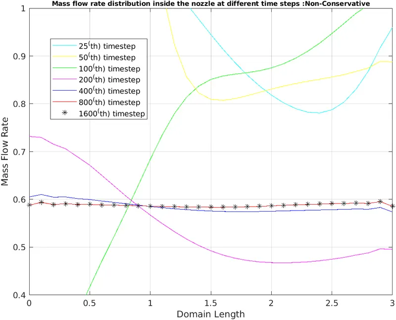
It appears that from the 400th timestep, the mass flow rate becomes stable along the domain length. Hence the 800th and 1600th timesteps coincide as the flow has become completely stable.
- Grid Independence test
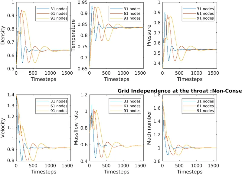
From the graphs we can see that after the solution becomes stable all the three lines coincide which mean that the mesh has become grid independent when n=31 nodes itself.
RESULTS: CONSERVATIVE FORM OF GOVERNING EQUATIONS
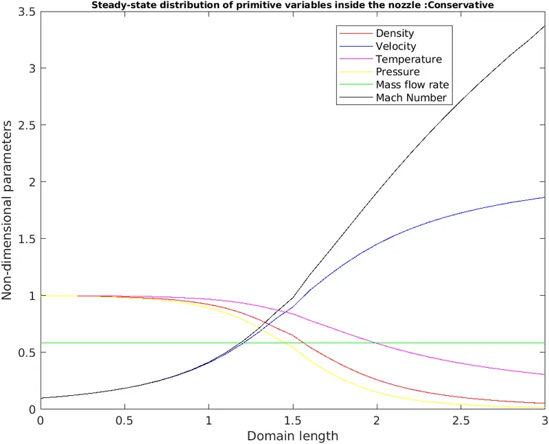
- Steady-state distribution of primitive variables inside the nozzle
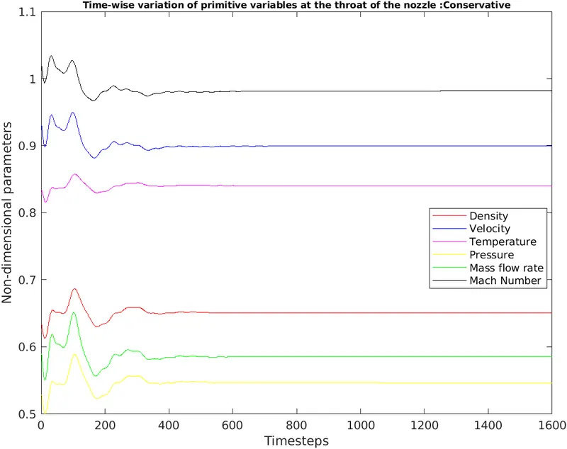
- Time-wise variation of the primitive variables
- Variation of Mass flow rate distribution inside the nozzle at different time steps during the time-marching process
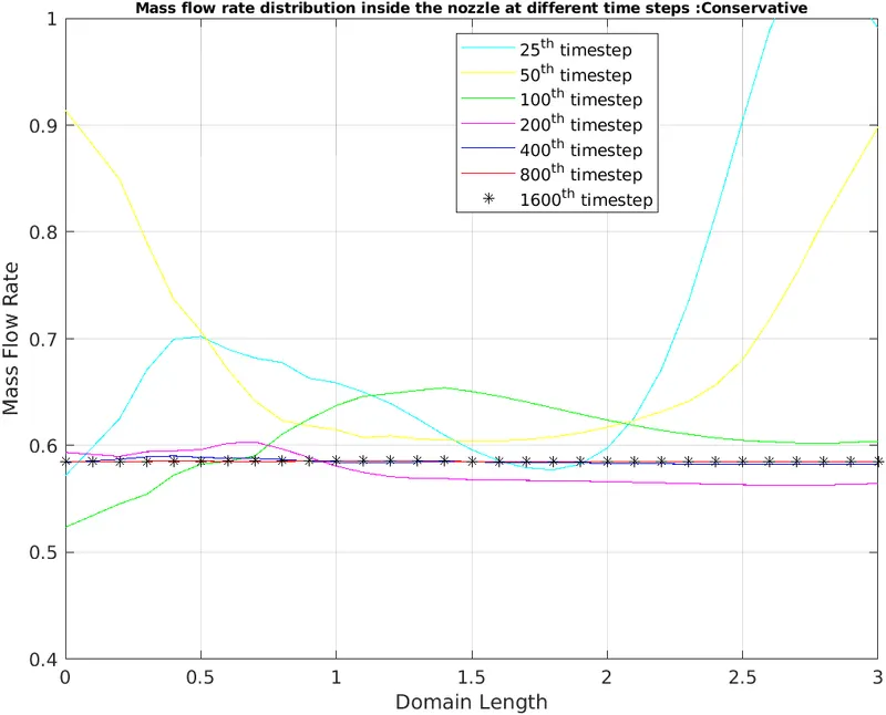
It appears that from the 200th timestep, the mass flow rate becomes stable along the domain length. Hence the 800th and 1600th timesteps coincide as the flow has become completely stable.
- Grid Independence test
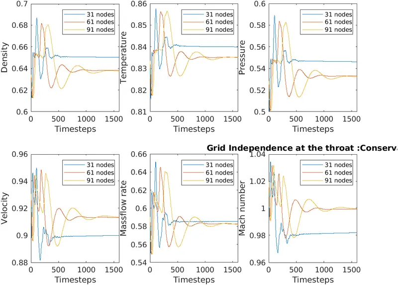
From the graphs we can see that after the solution becomes stable all the three lines are parallel to each other with a interline distance of the order of 1e-4, which mean that the mesh has become grid independent when n=31 nodes itself.
COMPARISON PLOT OF MASS FLOW RATE DISTRIBUTIONS OF BOTH FORMS