Solving the Steady and Unsteady/Transient 2D heat conduction problem under implicit and explicit schemes
OBJECTIVE
To solve the 2D heat conduction equation by using the point iterative techniques: Jacobi, Gauss-Siedel and Successive Over Relaxation (SOR) methods under implicit and explicit schemes for the transient and steady state cases with the boundary conditions for the problem as
Top Boundary = 600 K
Bottom Boundary = 900 K
Left Boundary = 400 K
Right Boundary = 800 K
We assume that all points in the inner part of the square domain is at a temperature of 300K.
The 2D heat conduction equation is given as `(dT)/(dt)=alpha((d^2T)/(dx^2)+(d^2T)/(dy^2))=alpha nabla^2T` where `alpha` is the thermal diffusivity.
Heat conduction can be of two kinds
- Steady state
- Transient state/Unsteady state
former means that it is independent of time and doesnot exist in the initial phases of real heat conduction cases. But every heat conduction scenario attains steady state after a specific number of iterations.
IMPLICIT SCHEME- STEADY STATE SCENARIO
The discretisation of steady state equation `(d^2T)/(dx^2)+(d^2T)/(dy^2)=0` can be done as
`(T_L-2T_P+T_R)/(Deltax^2)+(T_T-2T_P+T_B)/(Deltay^2)=0`
Here `Delta x=Delta y` so, `(T_L-2T_P+T_R+T_T-2T_P+T_B)/(Deltax^2)=0`
`T_L+T_R+T_T+T_B=4T_P`
`T_P=0.25(T_L+T_R+T_T+T_B)`
- Matlab Code: Jacobi, Gauss- Siedel and SOR iterations
% Code that solves steady state 2D conduction equation in implicit scheme
% -----------------------------------------------------------------------

  clear all
  close all
  clc

% Gridpoints and the conduction domain
   nx=10;
   ny=nx;
   x=linspace(0,1,nx);
   y=linspace(0,1,ny);
   dx=x(2)-x(1);
   dy=y(2)-y(1);

   iterator=[1,2,3];

% Defining boundary conditions for the domain
   T=300*ones(nx,ny);
   T_l=400;       % left side
   T_r=800;       % right side
   T_t=600;       % top
   T_b=900;       % bottom

   for k=iterator
       T(1,2:ny-1)=T_t;
       T(nx,2:ny-1)=T_b;
       T(2:nx-1,1)=T_l;
       T(2:nx-1,ny)=T_r;

    % Temperature at the corners
       T(1,1)=(T_t+T_l)/2;
       T(nx,1)=(T_b+T_l)/2;
       T(1,ny)=(T_t+T_r)/2;
       T(nx,ny)=(T_b+T_r)/2;

       T_initial=T;
       T_old=T;

    % error and tolerance
       Error=9e9;
       tol=1e-4;
       omega=2/(1+sin(pi*dx));

       if k==1
           % Solving by Jacobi Method
              Jac_iter=1;
              while (Error>tol)
                  for i=2:nx-1
                      for j=2:ny-1
                          T(i,j)=0.25*(T_old(i-1,j)+T_old(i+1,j)+T_old(i,j-1)+T_old(i,j+1));
                      end
                  end
                  Error=max(max(abs(T_old-T)));
                  T_old=T;
                  Jac_iter=Jac_iter+1;
              end
           % plotting
              figure(k)
              contourf(x,y,T)
              clabel(contourf(x,y,T))
              colorbar
              colormap(jet)
              set(gca,'ydir','reverse')
              xlabel('X-axis')
              ylabel('Y-axis')
              title(sprintf('Jacobi iterations in Implicit scheme in steady state= %d',Jac_iter))
              pause(0.003)
       end

       if k==2
           % Solving by Gauss-Siedel Method
              GS_iter=1;
              while (Error>tol)
                  for i=2:nx-1
                      for j=2:ny-1
                          T(i,j)=0.25*(T(i-1,j)+T_old(i+1,j)+T(i,j-1)+T_old(i,j+1));
                      end
                  end
                  Error=max(max(abs(T_old-T)));
                  T_old=T;
                  GS_iter=GS_iter+1;
              end
           % plotting
              figure(k)
              contourf(x,y,T)
              clabel(contourf(x,y,T))
              colorbar
              colormap(jet)
              set(gca,'ydir','reverse')
              xlabel('X-axis')
              ylabel('Y-axis')
              title(sprintf('Gauss-Siedel iterations in Implicit scheme at Steady state= %d',GS_iter))
              pause(0.003)
       end

       if k==3
           % Solving by SOR Method
              SOR_iter=1;
              while (Error>tol)
                  for i=2:nx-1
                      for j=2:ny-1
                          T(i,j)=omega*(0.25*(T(i-1,j)+T_old(i+1,j)+T(i,j-1)+T_old(i,j+1)))+(1-omega)*T_old(i,j);
                      end
                  end
                  Error=max(max(abs(T_old-T)));
                  T_old=T;
                  SOR_iter=SOR_iter+1;
              end
           % plotting
              figure(k)
              contourf(x,y,T)
              clabel(contourf(x,y,T))
              colorbar
              colormap(jet)
              set(gca,'ydir','reverse')
              xlabel('X-axis')
              ylabel('Y-axis')
              title(sprintf('SOR iterations in Implicit scheme at Steady state= %d',SOR_iter))
              pause(0.003)
       end
   end
- Results obtained
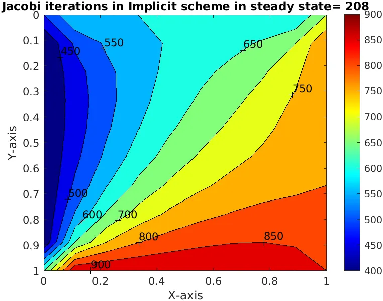
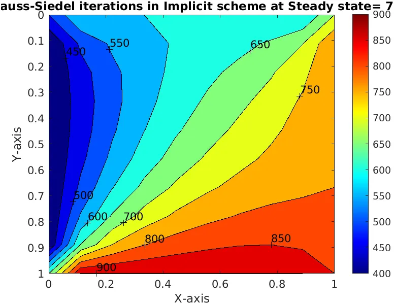
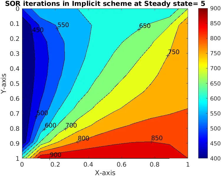
IMPLICIT SCHEME- UNSTEADY/TRANSIENT STATE SCENARIO
The discretisation of unsteady state equation `(dT)/(dt)=alpha((d^2T)/(dx^2)+(d^2T)/(dy^2))` can be done as
`(T_P^(n+1)-T_P^n)/(Deltat)=alpha((T_L-2T_P+T_R)/(Deltax^2)+(T_T-2T_P+T_B)/(Deltay^2))^(n+1)`
Let `k_1=alpha(Deltat)/(Deltax)` and `k_2=alpha(Deltat)/(Deltay)`
So on simplifying the above equation we get,
`T_P^(n+1)=(T_P^n+k_1(T_R+T_L)^(n+1)+k_2(T_T+T_B)^(n+1))/(1+2k_1+2k_2)`
- Matlab Code: Jacobi, Gauss- Siedel and SOR iterations
% Code that solves unsteady state 2D conduction equation in implicit scheme
% -------------------------------------------------------------------------

  clear all
  close all
  clc

% Gridpoints and the conduction domain
   nx=10;
   ny=nx;
   nt=2000;
   x=linspace(0,1,nx);
   y=linspace(0,1,ny);
   dx=x(2)-x(1);
   dy=y(2)-y(1);
   dt=1e-3;

   iterator=[1,2,3];

% Defining boundary conditions for the domain
   T=300*ones(nx,ny);
   T_l=400;       % left side
   T_r=800;       % right side
   T_t=600;       % top
   T_b=900;       % bottom

   for k=iterator
       T(1,2:ny-1)=T_t;
       T(nx,2:ny-1)=T_b;
       T(2:nx-1,1)=T_l;
       T(2:nx-1,ny)=T_r;

    % Temperature at the corners
       T(1,1)=(T_t+T_l)/2;
       T(nx,1)=(T_b+T_l)/2;
       T(1,ny)=(T_t+T_r)/2;
       T(nx,ny)=(T_b+T_r)/2;

       T_initial=T;
       T_old=T;

    % error and tolerance
       Error=9e9;
       tol=1e-4;
       omega=2/(1+sin(pi*dx));

    % Calculating individual terms for the conduction eqn
       k1=omega*dt/(dx)^2;
       k2=omega*dt/(dy)^2;

       if k==1
           % Solving by Jacobi Method
              Jac_iter=1;
              for a=1:nt
                Error=9e9;
                while (Error>tol)
                  for i=2:nx-1
                      for j=2:ny-1
                          term1=(1+2*k1+2*k2);
                          term2=k1/term1;
                          term3=k2/term1;
                          H=(T_old(i-1,j)+T_old(i+1,j));
                          V=(T_old(i,j-1)+T_old(i,j+1));

                          T(i,j)=T_old(i,j)/term1+H*term2+V*term3;
                      end
                  end
                  Error=max(max(abs(T_old-T)));
                  T_old=T;
                  Jac_iter=Jac_iter+1;
                end
              end

           % plotting
              figure(k)
              contourf(x,y,T)
              clabel(contourf(x,y,T))
              colorbar
              colormap(jet)
              set(gca,'ydir','reverse')
              xlabel('X-axis')
              ylabel('Y-axis')
              title(sprintf('Unsteady state Jacobi iterations in Implicit scheme= %d',Jac_iter))
              pause(0.003)
       end

       if k==2
           % Solving by Gauss-Siedel Method
              GS_iter=1;
              for a=1:nt
                Error=9e9;
                while (Error>tol)
                  for i=2:nx-1
                      for j=2:ny-1
                          term1=(1+2*k1+2*k2);
                          term2=k1/term1;
                          term3=k2/term1;
                          H=(T(i-1,j)+T_old(i+1,j));
                          V=(T(i,j-1)+T_old(i,j+1));

                          T(i,j)=T_old(i,j)/term1+H*term2+V*term3;
                      end
                  end
                  Error=max(max(abs(T_old-T)));
                  T_old=T;
                  GS_iter=GS_iter+1;
                end
              end
           % plotting
              figure(k)
              contourf(x,y,T)
              clabel(contourf(x,y,T))
              colorbar
              colormap(jet)
              set(gca,'ydir','reverse')
              xlabel('X-axis')
              ylabel('Y-axis')
              title(sprintf('Unsteady state Gauss-Siedel iterations in Implicit scheme= %d',GS_iter))
              pause(0.003)
       end

       if k==3
           % Solving by SOR Method
              SOR_iter=1;
              for a=1:nt
                Error=9e9;
                while (Error>tol)
                  for i=2:nx-1
                      for j=2:ny-1
                          term1=(1+2*k1+2*k2);
                          term2=k1/term1;
                          term3=k2/term1;
                          H=(T(i-1,j)+T_old(i+1,j));
                          V=(T(i,j-1)+T_old(i,j+1));

                          T(i,j)=omega*(T_old(i,j)/term1+H*term2+V*term3)+(1-omega)*T_old(i,j);
                      end
                  end
                  Error=max(max(abs(T_old-T)));
                  T_old=T;
                  SOR_iter=SOR_iter+1;
                end
              end
           % plotting
              figure(k)
              contourf(x,y,T)
              clabel(contourf(x,y,T))
              colorbar
              colormap(jet)
              set(gca,'ydir','reverse')
              xlabel('X-axis')
              ylabel('Y-axis')
              title(sprintf('Unsteady state SOR iterations in Implicit scheme= %d',SOR_iter))
              pause(0.003)
       end
   end
- Results obtained
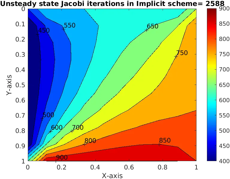
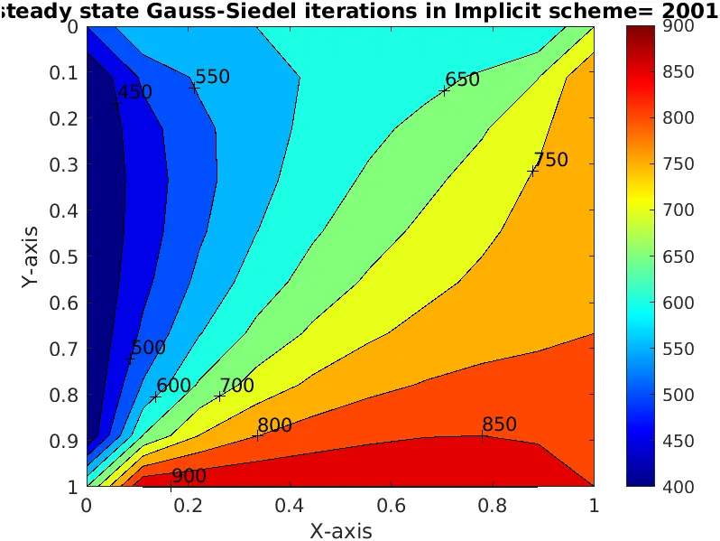
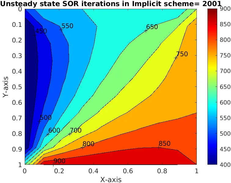
EXPLICIT SCHEME- UNSTEADY/TRANSIENT STATE SCENARIO
The discretisation of unsteady state equation `(dT)/(dt)=alpha((d^2T)/(dx^2)+(d^2T)/(dy^2))` can be done as
`(T_P^(n+1)-T_P^n)/(Deltat)=alpha((T_L-2T_P+T_R)/(Deltax^2)+(T_T-2T_P+T_B)/(Deltay^2))^n`
Let `k_1=alpha(Deltat)/(Deltax)` and `k_2=alpha(Deltat)/(Deltay)`
So on simplifying the above equation we get,
`T_P^(n+1)=T_P^n+k_1(T_L-2T_P+T_R)^n+k_2(T_T-2T_P+T_B)^n`
- Matlab Code: Explicit iterations
% Code that solves unsteady state 2D conduction equation in explicit scheme
% -------------------------------------------------------------------------

  clear all
  close all
  clc

% Gridpoints and the conduction domain
   nx=10;
   ny=nx;
   nt=2000;
   x=linspace(0,1,nx);
   y=linspace(0,1,ny);
   dx=x(2)-x(1);
   dy=y(2)-y(1);
   dt=1e-3;

% Defining boundary conditions for the domain
   T=300*ones(nx,ny);
   T_l=400;       % left side
   T_r=800;       % right side
   T_t=600;       % top
   T_b=900;       % bottom

   T(1,2:ny-1)=T_t;
   T(nx,2:ny-1)=T_b;
   T(2:nx-1,1)=T_l;
   T(2:nx-1,ny)=T_r;

% Temperature at the corners
   T(1,1)=(T_t+T_l)/2;
   T(nx,1)=(T_b+T_l)/2;
   T(1,ny)=(T_t+T_r)/2;
   T(nx,ny)=(T_b+T_r)/2;

   T_initial=T;
   T_old=T;

% error and tolerance
   Error=9e9;
   tol=1e-4;
   omega=2/(1+sin(pi*dx));

% Calculating individual terms for the conduction eqn
   k1=omega*dt/(dx)^2;
   k2=omega*dt/(dy)^2;

% Solving the heat conduction equation
   Explicit_iter=1;
   for a=1:nt
       Error=9e9;
       while (Error>tol)
           for i=2:nx-1
               for j=2:ny-1
                   term1=T_old(i,j);
                   term2=k1*(T_old(i-1,j)-2*T_old(i,j)+T_old(i+1,j));
                   term3=k2*(T_old(i,j-1)-2*T_old(i,j)+T_old(i,j+1));

                   T(i,j)=term1+term2+term3;
               end
           end
           Error=max(max(abs(T_old-T)));
           T_old=T;
           Explicit_iter=Explicit_iter+1;
       end
   end

% plotting
   figure(1)
   contourf(x,y,T)
   clabel(contourf(x,y,T))
   colorbar
   colormap(jet)
   set(gca,'ydir','reverse')
   xlabel('X-axis')
   ylabel('Y-axis')
   title(sprintf('Unsteady state iterations in Explicit scheme= %d',Explicit_iter))
pause(0.003) - Results obtained
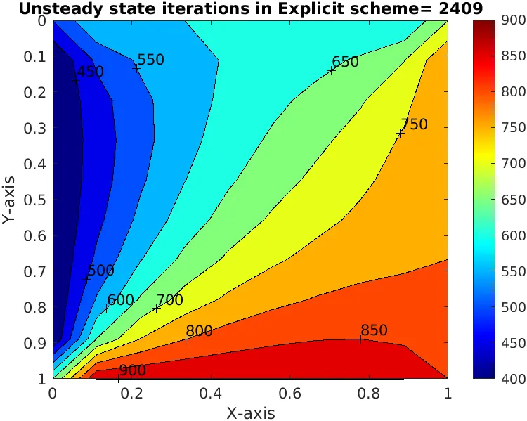
INFERENCE
Tabulating all the results we can see that,
| Type of scheme used | Iterative methods | No.of iterations |
| Implicit: Steady | Jacobi | 208 |
| Gauss Siedel | 7 | |
| Successive Over Relaxation | 5 | |
| Implicit: Transient | Jacobi | 2588 |
| Gauss Siedel | 2001 | |
| Successive Over Relaxation | 2001 | |
| Explicit: Transient | 2409 |
- Successive Over Relaxation is the most effective iteration method as it requires the least number of iterations to attain convergence in both Implicit and Explicit schemes
- Steady state analysis takes the least iterations to compute than the unsteady state