Challenge

Simulation of Hagen Poiseuille Flow through a pipe in OpenFoam using wedge boundary condition (Part 1/2)

AAndria Alex Thomas12 Oct 2021

OBJECTIVE

To simulate an axi-symmetric laminar flow by applying a wedge boundary condition. This is done because simulating the domain as a whole will increase the computational time and might not even complete the simulation if the system resources are scarce. The results obtained are validated with the Hagen- Poiseuille's equations for the fully developed flow.

PARAMETERS GIVEN AND TAKEN INTO ACCOUNT FOR

Reynolds number: `2100` (laminar flow)

Working fluid: water

Density: `1000` kg/m^3

Dynamic viscosity `mu` : `0.89text(x)10^-3` Pa.s

Kinematic viscosity `nu` : `10^-6` m^2/s

Assume diameter of pipe: `0.03` m

LAMINAR FLOW IN A PIPE

In a conduit completely filled with fluid, the flow occurs due to pressure difference. And due to the no slip boundary condition in a pipe, the velocity of fluid inside the pipe changes from zero at the walls and attains a maximum value at the centerline keeping the average flow of the pipe as constant as long as the area of cross-section doesnot change.

But as the velocity varies we observe a change in flow of fluid, ie., the flow transition occurs from laminar to turbulent. This transition is governed by the Reynolds number of the fluid flow. If `Re<=2100` the flow is laminar and if `Re>=4000` the flow is turbulent. The region in between undergoes a transition in flow. Here the flow is laminar as Re=2100.

Reynolds number `Re=(rhoV_(avg)D)/mu`

`:.` Average velocity `V_(avg)=Re*mu/(rho*D)=2100*0.00089/(1000*0.03)=0.0623m/s`

HYDRODYNAMIC ENTRY LENGTH

The region from the inlet of the pipe where the flow velocity boundary layer meets the centerline is called the hydrodynamic entrance length. The velocity profile is fully developed after the entrance length.

`:.` Hydrodynamic entry length for laminar flow `L_(h,l)=0.06*Re*D=0.06*2100*0.03=3.78m`

VELOCITY PROFILE OF THE FLOW

The profile is parabolic in nature for a fully developed flow where the maximum velocity is at the center line of the pipe.

The velocity profile `u(r)=R^2/(4mu)*((dp)/(dx))*(1-r^2/R^2)` and average velocity `V_(avg)=R^2/(8mu)*((dp)/(dx))`

`:.u(r)=2V_(avg)*(1-r^2/R^2)=0.1246*(1-r^2/R^2)`

SHEAR STRESS IN THE PIPE

Shear stress in a pipe can be formulated as `tau=mu*(du)/(dy)=mu*(du)/(dr)` in this case.

`(du(r))/(dr)=d/(dr)(2V_(avg)(1-r^2/R^2))=-(4V_(avg))/R^2r`

So, shear stress can be rewritten as `tau=-(4V_(avg))/R^2r*mu=-(4muV_(avg))/R^2r=k_1r implies` shear stress graph is a straight line graph.

Maximum shear stress would be at the walls ie, at r=R=0.015m

`tau_(max)=(4muV_(avg))/R=0.0148 Pa`

HAGEN POISEUILLE FLOW

Hagen Poiseuille flow gives the pressure drop in an incompressible and Newtonian fluid in laminar flow flowing through a long cylindrical pipe of constant cross section. It states that the pressure drop and the power required to induce the flow is directly proportional to the viscosity of the fluid and the length of the pipe for a constant flow rate but inversely proportional to the fourth power of the radius of the pipe.

Hence,

Maximum velocity `V_(max)=2V_(avg)=0.1246 m/s`
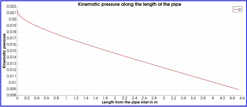
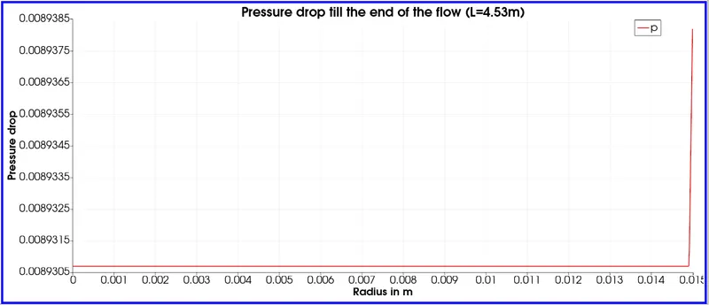
Pressure drop from Hagen Poiseulle equation `Delta P=(32muLV_(avg))/D^2=8.9307Pa`
Kinematic pressure `DeltaP_(text(kinematic))=(Delta P_(text(static)))/rho=0.0089307m`

MATLAB CODE

% Simulation of the flow through a pipe: wedge boundary condition
% ---------------------------------------------------------------

  clear all
  close all
  clc

% Parameters
  Re= 2100;            % Reynolds number
  D= 0.03;             % Diameter of pipe
  r= D/2;              % Radius
  rho= 1000;           % Density
  mu= 0.00089;         % Dynamic viscosity
  nu= mu/rho;          % Kinematic viscosity
  theta= 3;            % Wedge angle in degrees
  L_h= 0.06*Re*D;      % Hydrodynamic entrance length for laminar flow

% Boundary conditions
  L= L_h+0.75;         % Total length of pipe
  V_avg= Re*mu/(rho*D);% Average velocity
  V_max= 2*V_avg;      % Maximum velocity
  dp= 8*mu*L*V_avg/r^2;% Pressure

% Vertices
  y= r*cosd(theta/2);
  z= r*sind(theta/2);
  v0= [0 0 0];
  v1= [0 y -z];
  v2= [0 y z];
  v3= [L 0 0];
  v4= [L y -z];
  v5= [L y z];

  grading= 0.25;
  b1= 75;
  b2= 1;
  b3= 300;

% Creating bolckMeshDict file
  f1= fopen('blockMeshDict.txt','w');

  fprintf(f1,'%sn','/*--------------------------------*- C++ -*----------------------------------*');
  fprintf(f1,'%sn','  =========                 |');
  fprintf(f1,'%sn','  \      /  F ield         | OpenFOAM: The Open Source CFD Toolbox');
  fprintf(f1,'%sn','   \    /   O peration     | Website:  https://openfoam.org');
  fprintf(f1,'%sn','    \  /    A nd           | Version:  8');
  fprintf(f1,'%sn','     \/     M anipulation  |');
  fprintf(f1,'%snn','*---------------------------------------------------------------------------*/');

  fprintf(f1,'FoamFile n {n');
  fprintf(f1,'%16s %10s n','version','2.0;');
  fprintf(f1,'%16s %12s n','format','ascii;');
  fprintf(f1,'%16s %17s n','class','dictionary;');
  fprintf(f1,'%16s %20s n','object','blockMeshDict;');
  fprintf(f1,' }n');
  fprintf(f1,'%snn','// * * * * * * * * * * * * * * * * * * * * * * * * * * * * * * * * * * * * * //');

  fprintf(f1,'convertToMeters 1; n n');

  fprintf(f1,'vertices n (n');
  fprintf(f1,'t(%d %d %d)n',v0);
  fprintf(f1,'t(%d %d %d)n',v1);
  fprintf(f1,'t(%d %d %d)n',v2);
  fprintf(f1,'t(%d %d %d)n',v3);
  fprintf(f1,'t(%d %d %d)n',v4);
  fprintf(f1,'t(%d %d %d)n',v5);
  fprintf(f1,' ); nn');

  fprintf(f1,'blocks n (n');
  fprintf(f1,'t %s (%d %d %d) %s (%d 1 1)n','hex (0 1 2 0 3 4 5 3)',b1,b2,b3,'simpleGrading',grading);
  fprintf(f1,' ); nn');

  fprintf(f1,'edges n (n');
  fprintf(f1,'t %s(0 %d 0)n','arc 1 2',r);
  fprintf(f1,'t %s(%d %d 0)n','arc 4 5',L,r);
  fprintf(f1,' ); nn');

  fprintf(f1,'boundary n (n');
  fprintf(f1,'t%5sn','inlet','{');
  fprintf(f1,'t%12s %sn','type','patch;');
  fprintf(f1,'t%13sn %16sn','faces','(');
  fprintf(f1,'tt%14sn %17snn%13snn','(0 2 1 0)',');','}');

  fprintf(f1,'t%5sn','outlet','{');
  fprintf(f1,'t%12s %sn','type','patch;');
  fprintf(f1,'t%13sn %16sn','faces','(');
  fprintf(f1,'tt%14sn %17snn%13snn','(3 4 5 3)',');','}');

  fprintf(f1,'t%5sn','axis','{');
  fprintf(f1,'t%12s %sn','type','empty;');
  fprintf(f1,'t%13sn %16sn','faces','(');
  fprintf(f1,'tt%14sn %17snn%13snn','(0 3 3 0)',');','}');

  fprintf(f1,'t%5sn','wall','{');
  fprintf(f1,'t%12s %sn','type','wall;');
  fprintf(f1,'t%13sn %16sn','faces','(');
  fprintf(f1,'tt%14sn %17snn%13snn','(1 2 5 4)',');','}');

  fprintf(f1,'t%5sn','wedgefrontandback','{');
  fprintf(f1,'t%12s %sn','type','wedge;');
  fprintf(f1,'t%13sn %16sn','faces','(');
  fprintf(f1,'tt%14sntt%14sn %17snn%13snn','(0 3 5 2)','(0 1 4 3)',');','}');
  fprintf(f1,' ); nn');

  fprintf(f1,'mergePatchPairs n (n');
  fprintf(f1,' ); nn');

  fprintf(f1,'// ************************************************************************* //');
  fclose(f1);

% Plotting the analytical velocity profile
  R=linspace(0,r,16);
  U=2*V_avg*(1-((R.^2)/(r^2)));
  figure(1)
  plot(R,U,'b')
  hold on
  plot(-R,U,'b')
  hold on
  xlabel('Radius in m')
  ylabel('Velocity')
  title('Analytical Velocity profile at fully developed region','FontSize',9)

This MATLAB code generates a blockMeshDict file which will be used in our simulation. The solver used is icoFoam. This same method will be used to create a blockMeshDict file for wedge angle=4 degrees.

blockMeshDict file generated

/*--------------------------------*- C++ -*----------------------------------*
  =========                 |
  \      /  F ield         | OpenFOAM: The Open Source CFD Toolbox
   \    /   O peration     | Website:  https://openfoam.org
    \  /    A nd           | Version:  8
     \/     M anipulation  |
*---------------------------------------------------------------------------*/

FoamFile 
 {
         version       2.0; 
          format       ascii; 
           class       dictionary; 
          object       blockMeshDict; 
 }
// * * * * * * * * * * * * * * * * * * * * * * * * * * * * * * * * * * * * * //

convertToMeters 1; 
 
vertices 
 (
	(0 0 0)
	(0 1.499486e-02 -3.926542e-04)
	(0 1.499486e-02 3.926542e-04)
	(4.530000e+00 0 0)
	(4.530000e+00 1.499486e-02 -3.926542e-04)
	(4.530000e+00 1.499486e-02 3.926542e-04)
 ); 

blocks 
 (
	 hex (0 1 2 0 3 4 5 3) (75 1 300) simpleGrading (2.500000e-01 1 1)
 ); 

edges 
 (
	 arc 1 2 (0 1.500000e-02 0)
	 arc 4 5 (4.530000e+00 1.500000e-02 0)
 ); 

boundary 
 (
	inlet
	    {
	        type patch;
	        faces
                (
		     (0 2 1 0)
                );

            }

	outlet
	    {
	        type patch;
	        faces
                (
		     (3 4 5 3)
                );

            }

	 axis
	    {
	        type empty;
	        faces
                (
		     (0 3 3 0)
                );

            }

	walls
	    {
	        type wall;
	        faces
                (
		     (1 2 5 4)
                );

            }

	wedgefront
	    {
	        type wedge;
	        faces
                (
		     (0 3 5 2)
                );

            }

 ); 

	wedgeback
	    {
	        type wedge;
	        faces
                (
		     (0 1 4 3)
                );

            }

 ); 

mergePatchPairs 
 (
 ); 

// ************************************************************************* //

INITIAL CONDITIONS: Average velocity

/*--------------------------------*- C++ -*----------------------------------*
  =========                 |
  \      /  F ield         | OpenFOAM: The Open Source CFD Toolbox
   \    /   O peration     | Website:  https://openfoam.org
    \  /    A nd           | Version:  8
     \/     M anipulation  |
*---------------------------------------------------------------------------*/
FoamFile
{
    version     2.0;
    format      ascii;
    class       volVectorField;
    object      U;
}
// * * * * * * * * * * * * * * * * * * * * * * * * * * * * * * * * * * * * * //

dimensions      [0 1 -1 0 0 0 0];

internalField   uniform (0.0623 0 0);

boundaryField
{
    inlet
    {
        type            fixedValue;
        value           uniform (0.0623 0 0);
    }

    outlet
    {
        type            zeroGradient;
    }

    axis
    {
        type            empty;
    }

    wall
    {
        type            fixedValue;
        value           uniform (0 0 0);
    }


    wedgefront
    {
        type            wedge;
    }

    wedgeback
    {
        type            wedge;
    }
}

// ************************************************************************* //

INITIAL CONDITIONS: Pressure

/*--------------------------------*- C++ -*----------------------------------*
  =========                 |
  \      /  F ield         | OpenFOAM: The Open Source CFD Toolbox
   \    /   O peration     | Website:  https://openfoam.org
    \  /    A nd           | Version:  8
     \/     M anipulation  |
*---------------------------------------------------------------------------*/
FoamFile
{
    version     2.0;
    format      ascii;
    class       volScalarField;
    object      p;
}
// * * * * * * * * * * * * * * * * * * * * * * * * * * * * * * * * * * * * * //

dimensions      [0 2 -2 0 0 0 0];

internalField   uniform 0;

boundaryField
{
    inlet
    {
        type            zeroGradient;
    }

    outlet
    {
        type            fixedValue;
        value           uniform 0.0089307;
    }

    axis
    {
        type            empty;
    }

    wall
    {
        type            zeroGradient;
    }


    wedgefront
    {
        type            wedge;
    }

    wedgeback
    {
        type            wedge;
    }
}

// ************************************************************************* //

Transport properties: Kinematic Viscosity

/*--------------------------------*- C++ -*----------------------------------*
  =========                 |
  \      /  F ield         | OpenFOAM: The Open Source CFD Toolbox
   \    /   O peration     | Website:  https://openfoam.org
    \  /    A nd           | Version:  8
     \/     M anipulation  |
*---------------------------------------------------------------------------*/
FoamFile
{
    version     2.0;
    format      ascii;
    class       dictionary;
    location    "constant";
    object      transportProperties;
}
// * * * * * * * * * * * * * * * * * * * * * * * * * * * * * * * * * * * * * //

nu              [0 2 -1 0 0 0 0] 1e-06;


// ************************************************************************* //

ControlDict file

/*--------------------------------*- C++ -*----------------------------------*
  =========                 |
  \      /  F ield         | OpenFOAM: The Open Source CFD Toolbox
   \    /   O peration     | Website:  https://openfoam.org
    \  /    A nd           | Version:  8
     \/     M anipulation  |
*---------------------------------------------------------------------------*/
FoamFile
{
    version     2.0;
    format      ascii;
    class       dictionary;
    location    "system";
    object      controlDict;
}
// * * * * * * * * * * * * * * * * * * * * * * * * * * * * * * * * * * * * * //

application     icoFoam;

startFrom       startTime;

startTime       0;

stopAt          endTime;

endTime         50;

deltaT          0.005;

writeControl    timeStep;

writeInterval   200;

purgeWrite      0;

writeFormat     ascii;

writePrecision  6;

writeCompression off;

timeFormat      general;

timePrecision   6;

runTimeModifiable true;


// ************************************************************************* //

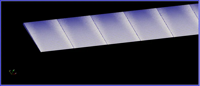
RESULTS FOR WEDGE ANGLE= 3 degrees

Mesh generated

Velocity distribution along the length from the inlet

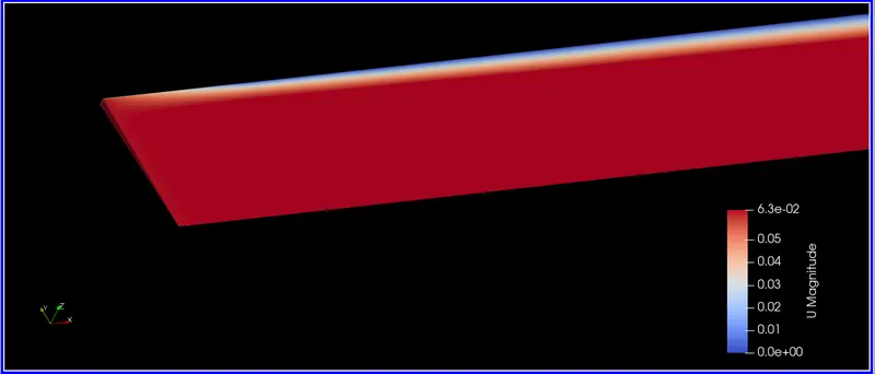
Velocity profiles

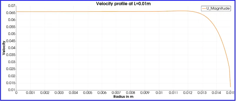
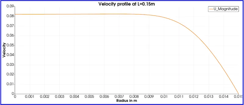
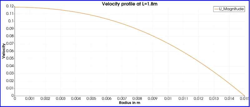
Velocity profile for fully developed flow

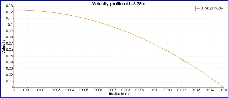
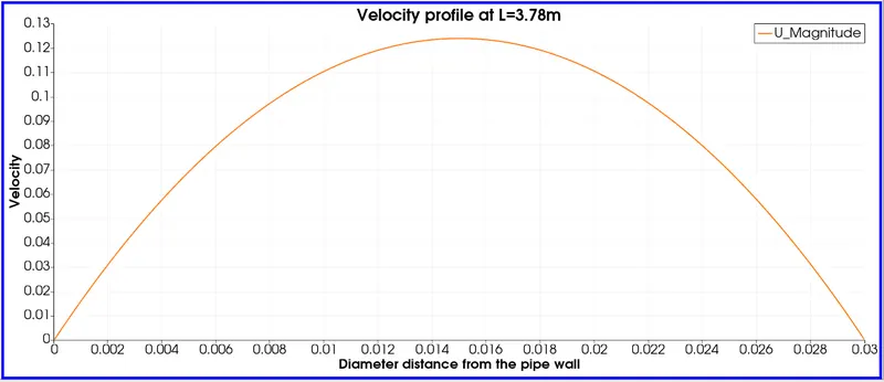
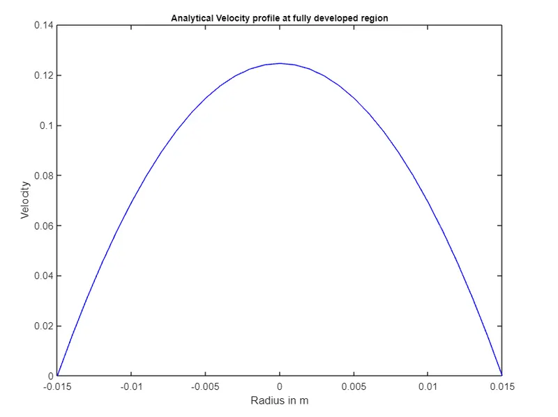
It is observed that after a certain point, the velocity profile remains the same and is independent of the length of the pipe. This point is the hydrodnamic entry length L=3.78m. On plotting the velocity graph analytically in MATLAB, we get the same results.

Kinematic Pressure

Shear stress distribution

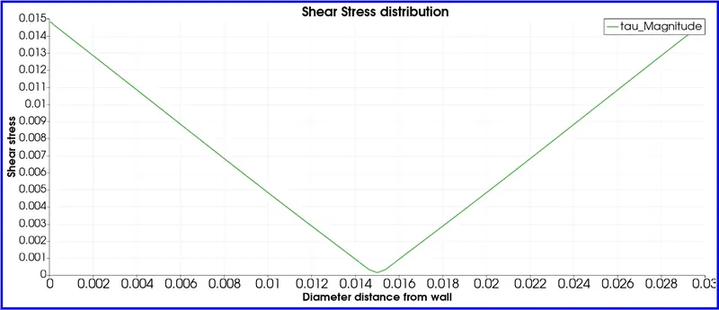
As expected, we got the shear stress plot to be linear and the stress increases from 0 in the center to their maximum values at the walls. The graph do satisfy the analytically calculated value of `tau_(max)=0.0148 Pa`.

COMPARISON WITH DIFFERENT WEDGE ANGLES

Wedge angle	Simulated value for velocity	Hagen Poiseuille value	Error
3	0.123963	0.1246	6.3700e-04
4	0.124124	0.1246	4.7600e-04

Simulation of Hagen Poiseuille Flow through a pipe in OpenFoam using wedge boundary condition (Part 1/2)

Ship work like this
in your own course.

Talk to a career counsellor

Ship work like thisin your own course.

Talk to a career counsellor

Ship work like this
in your own course.