Week 7 - Simulation of a 1D Super-sonic nozzle flow simulation using Macormack Method

OBJECTIVE :

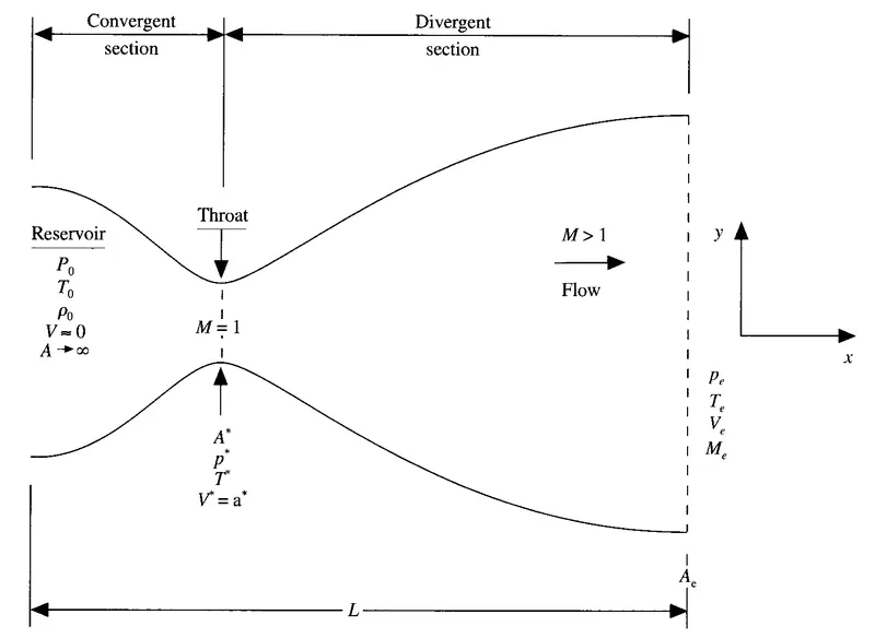
Simulate quasi 1 Directional flow through supersonic nozzle by solving governig equation in both conservative and non conservative form using MacCormacks technique.

Governing Equations :

Governing Equations are in terms of PDE for both Conservative and Non Conservative form in order to use Time Marching solution for the problem. These forms represent in numerical aspect only, if we analytic all the methods are same.

Conservative Form :

Continuity Equation

`(∂(ρA))/(∂t)+(∂(ρAv))/(∂x)=0`

Momentum Equation

`(∂(ρvA))/(∂t)+(∂(ρv^2 A))/(∂x)=-A (∂P)/(∂x)`

Energy Equation

`( ∂(ρ(e+v^2/2)A))/(∂t)+(∂(ρ(e+v^2/2)Av))/(∂x)=-(∂(PAv))/(∂x)`

Non Conservative Form :

Continuity Equation

`(∂(ρA))/(∂t)+ρA( ∂(v))/(∂x)+ρv (∂(A))/(∂x)+Av (∂(ρ))/(∂x)=0`

Momentum Equation

`ρ (∂v)/(∂t)+ρv (∂v)/(∂x)=-R(ρ (∂T)/(∂x )+T (∂ρ)/(∂x ))`

Energy Equation

`ρc_v (∂T)/(∂t)+ρvc_v (∂T)/(∂x)=-ρRT((∂v)/(∂x )+v (∂(lnA))/(∂x))`

Non Dimensionalising above equations

let

`T’= T /T_o`

`ρ’= ρ /ρ_o`

`x’= x /L`

`v’= v /a_`

`t’= t /(L/a_o)`

`A’= A / A^**`

Conservative Form:

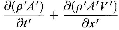
Continuity Equation

Momentum Equation

Energy Equation

Non Conservative Form :

Continuity Equation

Momentum Equation

Energy Equation

Maccorkmack Method:

This method is employed to solve the governing equations of quasi 1D supersonic nozzle flow rather than the differencing schemes as we have studied earlier.Maccorkmack method is an explicit finite difference technique which is second order accurate in both time and space. In CFD, the Maccorkmack method is a widely used discretization equations. This method essentially usues a predictor and corrector step.

Predictor Step

In this the spatial terms on the right-side of the equation are replaced by forward differences. The RHS of the eqn is known as all the variables are for time step 't. Next, the value of the LHS is calculated by employing the time marching solution and for the time-step 't-dt' values of the variable at all grid points is obtained.

Corrector Step

In this the spatial terms on the right-side of the equation are replaced by backward differences. The value of variables in RHS are taken which are obtained in the predicted step for time-step 't+dt.

Main Code :

clc
clear all
close all
n=31;
x=linspace(0,3,n);
dx=x(2)-x(1);
nt=1000;
C=0.5;
gamma=1.4;

% Solving for Non Conservatiove form
[rho_nc,v_nc,t_nc,Pressure_nc,Mass_Flow_Rate_nc,Mach_Number_nc,throat_nc,rho_throat_nc,v_throat_nc,t_throat_nc,Pressure_throat_nc,Mass_Flow_Rate_throat_nc,Mach_Number_throat_nc]=nonconservative_form(n,x,nt,C,dx,gamma);

% Plotting Variation of Properties with time step at throat
figure(2)
subplot(4,1,1)
plot(linspace(1,nt,nt),rho_throat_nc,'m');
ylabel('Density');
xlabel('Time Step Number');
title('Variation of Density at Throat in Non Conservative form');

subplot(4,1,2)
plot(linspace(1,nt,nt),t_throat_nc,'g');
ylabel('Temperature');
xlabel('Time Step Number');
title('Variation of Temperature at Throat in Non Conservative form');

subplot(4,1,3)
plot(linspace(1,nt,nt),Pressure_throat_nc,'r');
ylabel('Pressure');
xlabel('Time Step Number');
title('Variation of Pressureat Throat in Non Conservative form');


subplot(4,1,4)
plot(linspace(1,nt,nt),Mach_Number_throat_nc,'k');
ylabel('Mach Number');
xlabel('Time Step Number');
title('Variation of Mach Number at Throat in Non Conservative form');

% Steady State Solution for Non Conservative form

figure(3)
subplot(4,1,1)
plot(x,rho_nc,'m');
ylabel('Density');
xlabel('Nozzle Length');
title('Variation of Density for Non Conservative form');

subplot(4,1,2)
plot(x,t_nc,'g');
ylabel('Temperature');
xlabel('Nozzle Length');
title('Variation of Temperature for Non Conservative form');

subplot(4,1,3)
plot(x,Pressure_nc,'y');
ylabel('Pressure');
xlabel('Nozzle Length');
title('Variation of Pressure for Non Conservative form');


subplot(4,1,4)
plot(x,Mach_Number_nc,'r');
ylabel('Mach Number');
xlabel('Nozzle Length');
title('Variation of Mach Number for Non Conservative form');


% Conservative form
[rho_c,v_c,t_c,Pressure_c,Mass_Flow_Rate_c,Mach_Number_c,throat_c,rho_throat_c,v_throat_c,t_throat_c,Pressure_throat_c,Mass_Flow_Rate_throat_c,Mach_Number_throat_c]=conservative_form(n,x,nt,C,dx,gamma)

% Plotting Variation of Properties with time step at throat
figure(5)
subplot(4,1,1)
plot(linspace(1,nt,nt),rho_throat_c,'m');
ylabel('Density');
xlabel('Time Step Number');
title('Variation of Density at Throat in Conservative form');

subplot(4,1,2)
plot(linspace(1,nt,nt),t_throat_c,'g');
ylabel('Temperature');
xlabel('Time Step Number');
title('Variation of Temperature at Throat in Conservative form');

subplot(4,1,3)
plot(linspace(1,nt,nt),Pressure_throat_c,'r');
ylabel('Pressure');
xlabel('Time Step Number');
title('Variation of Pressureat Throat in Conservative form');


subplot(4,1,4)
plot(linspace(1,nt,nt),Mach_Number_throat_c,'k');
ylabel('Mach Number');
xlabel('Time Step Number');
title('Variation of Mach Number at Throat in Conservative form');

% Steady State Solution for Non Conservative form

figure(6)
subplot(4,1,1)
plot(x,rho_c,'m');
ylabel('Density');
xlabel('Nozzle Length');
title('Variation of Density for Conservative form');

subplot(4,1,2)
plot(x,t_c,'g');
ylabel('Temperature');
xlabel('Nozzle Length');
title('Variation of Temperature for Conservative form');

subplot(4,1,3)
plot(x,Pressure_c,'y');
ylabel('Pressure');
xlabel('Nozzle Length');
title('Variation of Pressure for Conservative form');


subplot(4,1,4)
plot(x,Mach_Number_c,'r');
ylabel('Mach Number');
xlabel('Nozzle Length');
title('Variation of Mach Number for Conservative form');

% Comparison of mass flow rate of conservative and non conservative form
figure(7)
plot(x,Mass_Flow_Rate_c,'r','linewidth',1.5);
hold on
plot(x,Mass_Flow_Rate_nc,'y','linewidth',1.5);
xlabel('Nozzle Length')
ylabel('Mass Flow Rate')
title('Comparison of flow rate for conservative and non conservative form')
legend('Conservative','Non Conservative')

Function for Conservative Form :

function [rho,v,t,Pressure,Mass_Flow_Rate,Mach_Number,throat,rho_throat,v_throat,t_throat,Pressure_throat,Mass_Flow_Rate_throat,Mach_Number_throat]=conservative_form(n,x,nt,C,dx,gamma)

% Initial Density and Temperature profile
for i=1:n
    if(x(i)>=0 && x(i)<=0.5)
        rho(i)=1;
        t(i)=1;
    elseif(x(i)>=0.5&& x(i)<=1.5)
        rho(i)=1-0.366*(x(i)-0.5);
        t(i)=1-0.167*(x(i)-0.5);
    elseif(x(i)>=1.5 && x(i)<=3)
        rho(i)=0.634-0.3879*(x(i)-1.5);
        t(i)=0.833-0.3507*(x(i)-1.5);
    end
end
% Area of Nozzle
a=1+2.2*(x-1.5).^2;
throat=find(a==1);

% Initial Velocity and Pressure
v=0.59./(rho.*a);
Pressure=rho.*t;

dt=min(C.*(dx./(sqrt(t)+v)));

% Initial Solution Vector
U1=rho.*a;
U2=rho.*a.*v;
U3=rho.*a.*((t/(gamma-1))+((gamma/2)*v.^2));

% Time loop
for k=1:nt
     % old values
     U1_old=U1;
     U2_old=U2;
     U3_old=U3;
     
     % Flux Vector
     F1=U2;
     F2=((U2.^2)./U1)+((gamma-1)/gamma).*(U3-((gamma/2)*((U2.^2)./U1)));
     F3=(gamma*((U2.*U3)./U1))-(gamma*(gamma-1)/2)*((U2.^3)./(U1.^2));
     
     % Predictor Method
     for j=2:n-1
     % Source Term
     J2(j)=(1/gamma)*rho(j)*t(j)*((a(j+1)-a(j))/dx);
     % Continuity equation
     dU1dt_p(j)=-((F1(j+1)-F1(j))/dx);
     
     % Momentum equation
    dU2dt_p(j)=-((F2(j+1)-F2(j))/dx)+J2(j);
    
    % Energy Equation
    dU3dt_p(j)=-((F3(j+1)-F3(j))/dx);
    
    % Upadate New Values
    U1(j)=U1(j)+dU1dt_p(j)*dt;
    U2(j)=U2(j)+dU2dt_p(j)*dt;
    U3(j)=U3(j)+dU3dt_p(j)*dt;
     end
    % Updating flux vector
     F1=U2;
     F2=((U2.^2)./U1)+((gamma-1)/gamma).*(U3-(gamma/2).*((U2.^2)./U1));
     F3=(gamma*((U2.*U3)./U1))-(gamma*(gamma-1)/2)*((U2.^3)./(U1.^2));
     
     % Primitive Values Update
    rho=U1./a;
    v=U2./U1;
    t=(gamma-1)*((U3./U1 - (gamma/2)*v.^2));
     
     % Corrector Method
     for j=2:n-1
         
         % Updating source term
        J2(j)=(1/gamma)*rho(j)*t(j)*((a(j)-a(j-1))/dx);
        
     % Continuity equation
     dU1dt_c(j)=-((F1(j)-F1(j-1))/dx);
     
     % Momentum equation
    dU2dt_c(j)=-((F2(j)-F2(j-1))/dx)+J2(j);
    
    % Energy Equation
    dU3dt_c(j)=-((F3(j)-F3(j-1))/dx);
       
     end
     
     % Average Time Derivative
     dU1dt=0.5*(dU1dt_p+dU1dt_c);
     dU2dt=0.5*(dU2dt_p+dU2dt_c);
     dU3dt=0.5*(dU3dt_p+dU3dt_c);
     
     % Solution Update
     for j=2:n-1
    U1(j)=U1_old(j)+dU1dt(j)*dt;
    U2(j)=U2_old(j)+dU2dt(j)*dt;
    U3(j)=U3_old(j)+dU3dt(j)*dt;
     end
     
     % Boudary Conditions
     % Inlet
     U1(1)=rho(1)*a(1);
     U2(1)=2*U2(2)-U2(3);
     v(1)=U2(1)/U1(1);
     U3(1)=U1(1)*((t(1)/(gamma-1))+(gamma/2)*v(1)^2);
     
     %Outlet
     U1(n)=2*U1(n-1)-U1(n-2);
     U2(n)=2*U2(n-1)-U2(n-2);
     U3(n)=2*U3(n-1)-U3(n-2);
     
    %  Final Primitive Values Update
    rho=U1./a;
    v=U2./U1;
    t=(gamma-1)*((U3./U1 - (gamma/2)*(v.^2)));
    
     % Mass flow rate , Pressure and Mach number calculation
    Mass_Flow_Rate=rho.*v.*a;
    Pressure=rho.*t;
    Mach_Number=(v./sqrt(t));
    
    rho_throat(k)=rho(throat);
    v_throat(k)=v(throat);
    t_throat(k)=t(throat);
    Mass_Flow_Rate_throat(k)=Mass_Flow_Rate(throat);
    Pressure_throat(k)=Pressure(throat);
    Mach_Number_throat(k)=Mach_Number(throat);
    
    
    % Plotting Graphs
    figure(4)
    if k==50
        plot(x,Mass_Flow_Rate,'r','linewidth',1.5)
        hold on
    elseif k==100
        plot(x,Mass_Flow_Rate,'b','linewidth',1.5)
        hold on
    elseif k==150
        plot(x,Mass_Flow_Rate,'c','linewidth',1.5)
        hold on
    elseif k==200
        plot(x,Mass_Flow_Rate,'y','linewidth',1.5)
        hold on
     elseif k==500
        plot(x,Mass_Flow_Rate,'g','linewidth',1.5)
        hold on      
     elseif k==1000
        plot(x,Mass_Flow_Rate,'k','linewidth',1.5)
        ylabel('Mass Flow Rate');
        xlabel('Nozzle Length');
        title('Mass Flow Rate at Different Time Steps for conservative form');
        legend('50','100','150','200','500','1000');
        
    end
        
end
    

Function for Non Conservative form :

function [rho,v,t,Pressure,Mass_Flow_Rate,Mach_Number,throat,rho_throat,v_throat,t_throat,Pressure_throat,Mass_Flow_Rate_throat,Mach_Number_throat]=nonconservative_form(n,x,nt,C,dx,gamma)
% initial profile
rho=1-0.3146*x;
t=1-0.2341*x;
v=(0.1+1.09*x).*t.^0.5;
a=1+2.2*(x-1.5).^2;
throat=find(a==1);
dt=min(C*(dx./(sqrt(t)+v)));
% outer time loop
for k=1:nt
    rho_old=rho;
    v_old=v;
    t_old=t;
    
    % Predictor method
    
    for j=2:n-1
        dvdx=(v(j+1)-v(j))/dx;
        drhodx=(rho(j+1)-rho(j))/dx;
        dtdx=(t(j+1)-t(j))/dx;
        dlogadx=(log(a(j+1))-log(a(j)))/dx;
         % continuity eqation
        drhodt_p(j)=-rho(j)*dvdx -rho(j)*v(j)*dlogadx-v(j)*drhodx;
        % momentum equation
        dvdt_p(j)=-v(j)*dvdx-(1/gamma)*(dtdx+(t(j)/rho(j))*drhodx);
        % Energy equation
        dtdt_p(j)=-v(j)*dtdx-(gamma-1)*t(j)*(dvdx+v(j)*dlogadx);
        
        % Solution update
        rho(j)=rho(j)+drhodt_p(j)*dt;
        v(j)=v(j)+dvdt_p(j)*dt;
        t(j)=t(j)+dtdt_p(j)*dt;
    end
    
     % Predictor method
    
    for j=2:n-1
        dvdx=(v(j)-v(j-1))/dx;
        drhodx=(rho(j)-rho(j-1))/dx;
        dtdx=(t(j)-t(j-1))/dx;
        dlogadx=(log(a(j))-log(a(j-1)))/dx;
         % continuity eqation
        drhodt_c(j)=-rho(j)*dvdx -rho(j)*v(j)*dlogadx-v(j)*drhodx;
        % momentum equation
        dvdt_c(j)=-v(j)*dvdx-(1/gamma)*(dtdx+(t(j)/rho(j))*drhodx);
        % Energy equation
        dtdt_c(j)=-v(j)*dtdx-(gamma-1)*t(j)*(dvdx+v(j)*dlogadx);
    end
    
    % Average time derivative
    drhodt=0.5*(drhodt_p+drhodt_c);
    dvdt=0.5*(dvdt_p+dvdt_c);
    dtdt=0.5*(dtdt_p+dtdt_c);
    
    % Final Solution Update
    for i=2:n-1
    rho(i)=rho_old(i)+drhodt(i)*dt;
    v(i)=v_old(i)+dvdt(i)*dt;
    t(i)=t_old(i)+dtdt(i)*dt;
    end
    
    % Applying Boundary conditions
    % Inlet BC
    rho(1)=1;
    v(1)=2*v(2)-v(3);
    t(1)=1;
   % Outlet BC
   rho(n)=2*rho(n-1)-rho(n-2);
    v(n)=2*v(n-1)-v(n-2);
    t(n)=2*t(n-1)-t(n-2);
    % Mass flow rate , Pressure and Mach number calculation
    Mass_Flow_Rate=rho.*v.*a;
    Pressure=rho.*t;
    Mach_Number=(v./sqrt(t));
    
    rho_throat(k)=rho(throat);
    v_throat(k)=v(throat);
    t_throat(k)=t(throat);
    Mass_Flow_Rate_throat(k)=Mass_Flow_Rate(throat);
    Pressure_throat(k)=Pressure(throat);
    Mach_Number_throat(k)=Mach_Number(throat);
    
    
    % Plotting Graphs
    figure(1)
    if k==50
        plot(x,Mass_Flow_Rate,'r','linewidth',1.5)
        hold on
    elseif k==100
        plot(x,Mass_Flow_Rate,'b','linewidth',1.5)
        hold on
    elseif k==150
        plot(x,Mass_Flow_Rate,'c','linewidth',1.5)
        hold on
    elseif k==200
        plot(x,Mass_Flow_Rate,'y','linewidth',1.5)
        hold on
     elseif k==500
        plot(x,Mass_Flow_Rate,'g','linewidth',1.5)
        hold on      
     elseif k==1000
        plot(x,Mass_Flow_Rate,'k','linewidth',1.5)
        ylabel('Mass Flow Rate');
        xlabel('Nozzle Length');
        title('Mass Flow Rate at Different Time Steps for non conservative form');
        legend('50','100','150','200','500','1000');
        
    end
   
end
    

Results :

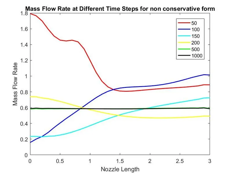
In above figure we can see after nearly 500 time steps mass flow rate becomes constant that it reaches steady state.

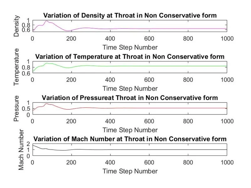
Above graphs shows Pressure , Temperature and Density becomes steady at throat section after nearly 500 time steps. Mach number also becomes 1 and remains constat.

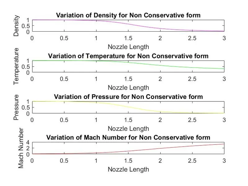
Above graph shows the variation of different variables with nozzle length.

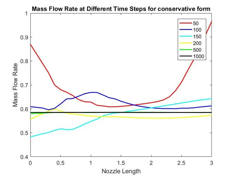
Above graph shows for non conservative approach mass flow rate becomes constant at every section in nozzle after some 500 time steps.

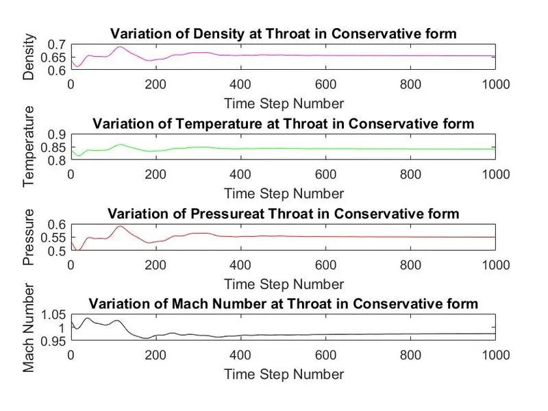
Above graph shows variation of different properties with number of time steps at throat section.

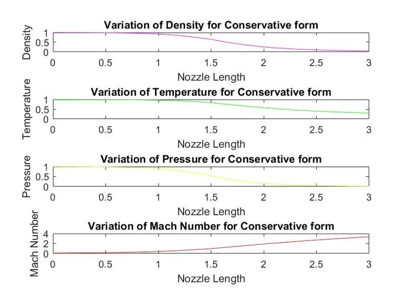
Above graph show variation of different variables with nozzle length after reaching steady state.

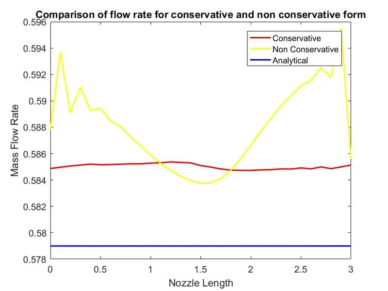
Above graph shows conservative approach give smooth solution compare to non conservative approach. Conservative approach gives slution nearer to Analytical at every section but non conservative solution is close to analytical one at the throat section only. We can say conservative form conserves mass better.

Grid Independent Study :

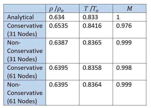
From above table we can say that Conservative form requires more number of calculations compare to Non conservative form for same accuracy.