Week 5.1 - Mid term project - Solving the steady and unsteady 2D heat conduction problem

Objective : 

 To solve the 2D heat conduction equation by using the point iterative techniques like Jacobi, Gauss-seidel and Successive over-relaxation (SOR).

Given Data :

The Boundary conditions for the problem are as follows

Top Boundary = 600 K

Bottom Boundary = 900 K

Left Boundary = 400 K

Right Boundary = 800 K.

Case 1 : Steady state 2D conduction equation.

`(∂^2 T)/(∂x^2 )+(∂^2 T)/(∂y^2 )=0`

Above steady state equation is elliptic in nature so we have to take information from all the directions thus we will use central difference method for discretization.

`T(i,j)=1/K ((T(i-1,j)+T(i+1,j))/(Δx^2 ))+1/K ((T(i,j-1)+T(i,j+1))/(Δy^2 ))`

where `K=2((Δx^2+Δy^2 )/(Δx^2 Δy^2 ))`

1. Solving using jacobi method :

In this method for finding the value of T at current iteration we have take values of all surrounding nodes at  previous iteration .

`T(i,j)=1/K ((T__old(i-1,j)+T__old(i+1,j))/(Δx^2 ))+1/K ((T__old(i,j-1)+T__old(i,j+1))/(Δy^2 ))`

2. Solving using Gauss Seidal Method :

In this method for finding the value of T at current iteration we have take values of preciding  nodes at  previous iteration and suceeding nodes at the current itteration.

`T(i,j)=1/K ((T__old(i-1,j)+T(i+1,j))/(Δx^2 ))+1/K ((T__old(i,j-1)+T(i,j+1))/(Δy^2 ))`

3. Solving using Successive over-relaxation (SOR).

In this method we use relaxation parameter to improve the convergence characteristic of oterative method. Here we multiply relaxatiion parameter by residual and add it to value at previous itteration. 

`T(i,j)=(1-w)(T__old(i,j))+w(1/K ((T__old(i-1,j)+T(i+1,j))/(Δx^2 ))+1/K ((T__old(i,j-1)+T(i,j+1))/(Δy^2 )))`

Where w is relaxation factor if w>1 then it is called over relaxation method and if w<1 then it is called under relaxation method. 

Code for Steady state condition:

close all 
clear all
clc
% Inpute parameters
nx=10;                   % No. of grid points in x direction
ny=10;                   % No. of grid points in x direction
x=linspace(0,1,nx);
y=linspace(0,1,ny);
dx=x(2)-x(1);
dy=y(2)-y(1);
% Boundary conditions
T_L=400;
T_R=800;
T_T=600;
T_B=900;
% Taking initial guess for temperature i.e. T=400 K
T=400*ones(nx,ny); 
% Defining temperature at edges
T(1,2:nx-1)=T_T;
T(ny,2:nx-1)=T_B;
T(2:ny-1,1)=T_L;
T(2:ny-1,nx)=T_R;
% Defining temperature at corners
T(1,1)=(T_L+T_T)/2;
T(1,nx)=(T_T+T_R)/2;
T(ny,1)=(T_L+T_B)/2;
T(ny,nx)=(T_B+T_R)/2;

T_old=T;                             % Defining Value of T at previous iteration
T_initial=T;                         % DEfining values of T at previous time step
K=2*(dx^2 + dy^2 )/(dx^2 * dy^2 );
tolerance=1e-4;                      % defining tolerance 
error=9e9;

iterative_solver=3;                  % choosing solver type 1 for jacobu, 2 for GS and 3 for SOR

% Jacobi Method

if iterative_solver==1
    jacobi_iteration=1;
   
    while(error > tolerance)
      % space loop start  
        for i=2:ny-1                                     
            for j=2:nx-1
                T(i,j)=(1/(K*dx^2))*(T_old(i+1,j)+T_old(i-1,j)+T_old(i,j+1)+T_old(i,j-1));
            end
        end
       % space loop end
        error=max(max(abs(T_old-T)));
        T_old=T;                                % updating old values 
        jacobi_iteration=jacobi_iteration+1;
    end
    contourf(x,y,T);                            % plotting contour 
clabel(contourf(x,y,T));
colorbar;
colormap(jet);
set(gca,'ydir','reverse');
title(sprintf('No. of jacobi iteration = %d ', jacobi_iteration));
xlabel('X-axis');
ylabel('Y-axis');
pause(0.03) ;  
end
     
        
% Gauss-Seidal Methoid
if iterative_solver==2
     GS_iteration=1;
   
    while(error > tolerance)
        % space loop start
        for i=2:ny-1
            for j=2:nx-1
                T(i,j)=(1/(K*dx^2))*(T_old(i+1,j)+T(i-1,j)+T_old(i,j+1)+T(i,j-1));
            end
        end
       % space loop end
        error=max(max(abs(T_old-T))); % calculation updated error
        T_old=T;                      % updation old values
        GS_iteration=GS_iteration+1;
    end
    contourf(x,y,T);                  % plotting contours
clabel(contourf(x,y,T));
colorbar;
colormap(jet);
set(gca,'ydir','reverse');
title(sprintf('No. of Gauss seidal iteration = %d ', GS_iteration));
xlabel('X-axis');
ylabel('Y-axis');
pause(0.03) ;             
end

% SOR  Methoid
if iterative_solver==3
    w=1.5;                % Relaxation paramter
     SOR_iteration=1;
   
    while(error > tolerance)
        % space loop start
        for i=2:ny-1
            for j=2:nx-1
                T(i,j)=(1-w)*T_old(i,j)+(w*((1/(K*dx^2))*(T_old(i+1,j)+T(i-1,j)+T_old(i,j+1)+T(i,j-1))));
            end
        end
        % Space loop end
        error=max(max(abs(T_old-T)));  % updating error
        T_old=T;                       % updating old values
        SOR_iteration=SOR_iteration+1;
    end
    contourf(x,y,T);                   % Plotting contours
clabel(contourf(x,y,T));
colorbar;
colormap(jet);
set(gca,'ydir','reverse');
title(sprintf('No. of SOR iteration = %d ', SOR_iteration));
xlabel('X-axis');
ylabel('Y-axis');
pause(0.03) ;             
end

Results : 

1.

2.

3.

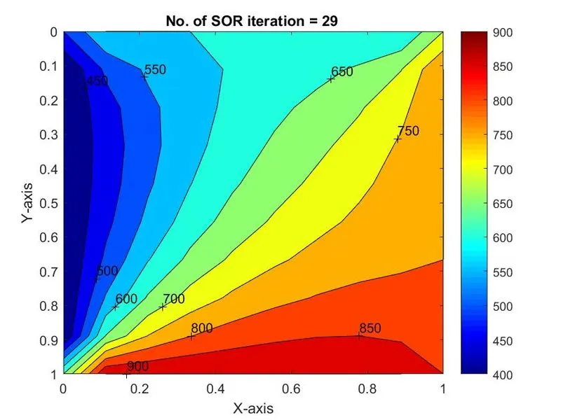
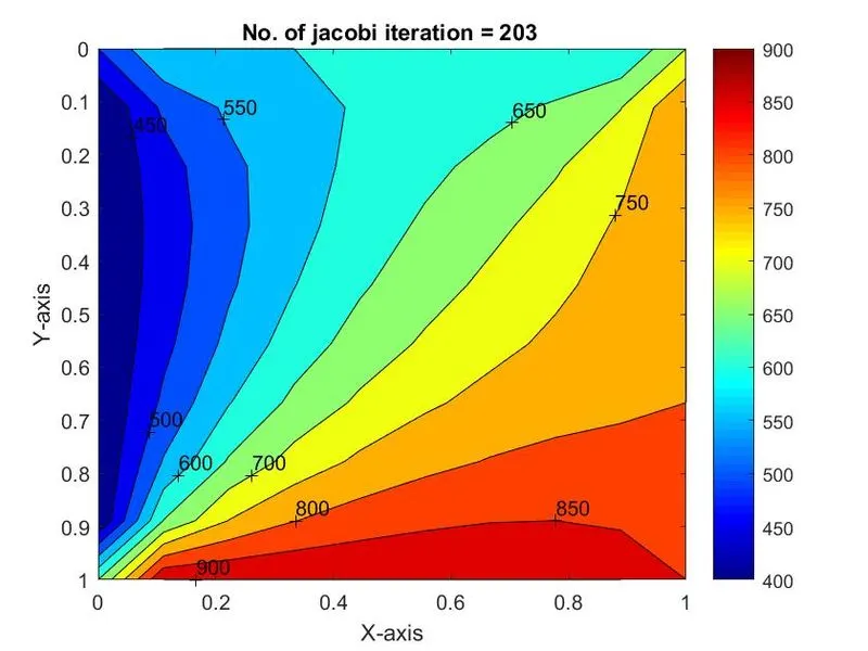
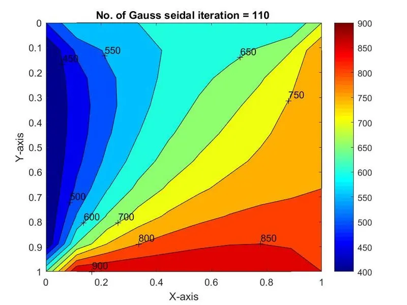
From the the above graphs it can be seen that the number of iteration required for jacobi is greater than gauss seidal and iteration for gauss seidal is greater than SOR. Thus we can say SOR can converge faster if proper relaxation parameter is considered.

Case 2. Unsteady / Transient 2D conduction problem

`(∂T)/(∂t)=α((∂^2 T)/(∂x^2 )+(∂^2 T)/(∂y^2 ))`

Explicit Method :

Here we will use all the information from previous iteration to calculate the value at present iteration.

Discretised equation by explicit method is given as

`(T_(i,j)^(n+1)-T_(i,j)^n)/(Δt)=α((T_(i+1,j)^(n)-2T_(i,j)^n+T_(i-1,j)^n)/(Δx^2) + (T_(i,j+1)^(n)-2T_(i,j)^n+T_(i,j+1)^n)/(Δy^2 ))`

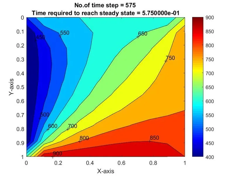
where 'α' is thermal diffusivity which indicate how fast heat will diffuse and object reach to steady state. 

Code for Unsteady Explicit:

close all 
clear all
clc
% Inpute parameters
nx=10;                   % No. of grid points
ny=10;
dt=0.001;
x=linspace(0,1,nx);
y=linspace(0,1,ny);
dx=x(2)-x(1);           % Length of element
dy=y(2)-y(1);
% Boundary conditions
T_L=400;
T_R=800;
T_T=600;
T_B=900;
T=400*ones(nx,ny);      % Taking initial guess for temperature
% Defining temperature at edges.
T(1,2:nx-1)=T_T;
T(ny,2:nx-1)=T_B;
T(2:ny-1,1)=T_L;
T(2:ny-1,nx)=T_R;
% defining temperature at corners
T(1,1)=(T_L+T_T)/2;
T(1,nx)=(T_T+T_R)/2;
T(ny,1)=(T_L+T_B)/2;
T(ny,nx)=(T_B+T_R)/2;
alpha=1;             % thermal duffusivity
T_old=T;
T_initial=T;
K1=(alpha*dt)/dx^2;
K2=(alpha*dt)/dy^2;
tolerance=1e-4;       % giving tolerance or required residual 
error=9e9;
 % time loop
for k=1:1400
    % space loop
        for i=2:ny-1
            for j=2:nx-1
                T(i,j)=T_old(i,j)+K1*(T_old(i+1,j)-2*T_old(i,j)+T_old(i-1,j))+K2*(T_old(i,j+1)-2*T_old(i,j)+T_old(i,j-1));
            end
        end
        % space loop end
        error=max(max(abs(T_old-T)));
        T_old=T;                      % updating old values
         Time_step=k;
         Time=k*dt;
      contourf(x,y,T);   % Plotting Contour at every time steps
clabel(contourf(x,y,T));
colorbar;
colormap(jet);
set(gca,'ydir','reverse');
xlabel('X-axis');
ylabel('Y-axis');
title(sprintf('No.of time step = %d \n Time required to reach steady state = %d sec ', Time_step,Time));
 pause(0.03) 
 if error< tolerance
     break
 end
end
% Time loop ends
     

Emplicit Method :

Here to calculate infirmation at current time step instead of taking information from previous time step we assume information at same time step.

Discretized equation by implicit method

`(T_(i,j)^(n+1)-T_(i,j)^n)/(Δt)=α((T_(i+1,j)^(n+1)-2T_(i,j)^(n+1)+T_(i-1,j)^(n+1))/(Δx^2) + (T_(i,j+1)^(n+1)-2T_(i,j)^(n+1)+T_(i,j+1)^(n+1))/(Δy^2 ))`

Jacobi Method:

`T_(i,j)^(n+1)=1/((1+2k_1+2k_2 ) )(T_(i,j)^n+k_1 (T__old_(i+1,j)^(n+1)+T__old_(i-1,j)^(n+1) )+k_2 (T__old_(i,j+1)^(n+1)+T__old_(i,j-1)^(n+1) )`

where `k_1=(α Δt)/(Δx^2 )` 

and     `k_2=(α Δt)/(Δy^2 )`

Gauss Seidal Method :

`T_(i,j)^(n+1)=1/((1+2k_1+2k_2 ) )(T_(i,j)^n+k_1 (T__old_(i+1,j)^(n+1)+T_(i-1,j)^(n+1) )+k_2 (T__old_(i,j+1)^(n+1)+T_(i,j-1)^(n+1) )`

SOR Method :

`T_(i,j)^(n+1)=(1-w)T__old_(i,j)^(n+1)+w(1/((1+2k_1+2k_2 ) )(T_(i,j)^n+k_1 (T__old_(i+1,j)^(n+1)+T_(i-1,j)^(n+1) )+k_2 (T__old_(i,j+1)^(n+1)+T_(i,j-1)^(n+1) ))`

where w is relaxation parameter

Code for Implicit method : 

close all 
clear all
clc
% Inpute parameters
nx=10;                   % No. of grid points
ny=10;
dt=0.001;
alpha=1;
w=1.1;
x=linspace(0,1,nx);
y=linspace(0,1,ny);
dx=x(2)-x(1);           % length of element or grid size
dy=y(2)-y(1);
% Boundary conditions
T_L=400;
T_R=800;
T_T=600;
T_B=900;
T=400*ones(nx,ny);        % initial guess for temperature
% defining boundary conditions at edges
T(1,2:nx-1)=T_T;
T(ny,2:nx-1)=T_B;
T(2:ny-1,1)=T_L;
T(2:ny-1,nx)=T_R;
% defining boundary conditions at corners
T(1,1)=(T_L+T_T)/2;
T(1,nx)=(T_T+T_R)/2;
T(ny,1)=(T_L+T_B)/2;
T(ny,nx)=(T_B+T_R)/2;

T_old=T;             % defining values at previous iteration
T_initial=T;             % defining values at previous time step
K1=(alpha*dt)/dx^2;
K2=(alpha*dt)/dy^2;
tolerance=1e-4;     % Giving tolerance or required residual
error=9e9;

iterative_solver=3;

% Jacobi Method

if iterative_solver==1
 jacobi_iteration=1;   
   for t=1:1400   % time loop
       error=9e9; 
    while(error > tolerance)   
        for i=2:ny-1         % space loop
            for j=2:nx-1
                T(i,j)=(1/(1+2*K1+2*K2))*(T_initial(i,j)+K1*(T_old(i+1,j)+T_old(i-1,j))+K2*(T_old(i,j+1)+T_old(i,j-1)));
            end
        end
        error=max(max(abs(T_old-T))); % calculating updated error
        T_old=T;                      % upodating old values
        jacobi_iteration=jacobi_iteration+1;
    end
    T_initial=T;                      % updating values at previous time step
    contourf(x,y,T);                   % plotting contour at each time step
clabel(contourf(x,y,T));
colorbar;
colormap(jet);
set(gca,'ydir','reverse');
title(sprintf('No. of jacobi iteration = %d \n No. of tome steps = %d', jacobi_iteration,t));
xlabel('X-axis');
ylabel('Y-axis'); 
pause(0.03)
   end
end

% Gauss Seidal
if iterative_solver==2
 GS_iteration=1;   
   for t=1:1400  % time loop
       error=9e9; 
    while(error > tolerance)   
        for i=2:ny-1      % space loop 
            for j=2:nx-1
                T(i,j)=(1/(1+2*K1+2*K2))*(T_initial(i,j)+K1*(T_old(i+1,j)+T(i-1,j))+K2*(T_old(i,j+1)+T(i,j-1)));
            end
        end
        error=max(max(abs(T_old-T))); % updating error
        T_old=T;                        % updating old values
        GS_iteration=GS_iteration+1;
    end
    T_initial=T;                      % updating values at previous time steps
    contourf(x,y,T);                  % plotting contours at each time step
clabel(contourf(x,y,T));
colorbar;
colormap(jet);
set(gca,'ydir','reverse');
title(sprintf('No. of Gauss Seidal iteration = %d \n No. of time steps = %d', GS_iteration,t));
xlabel('X-axis');
ylabel('Y-axis'); 
pause(0.03)
   end
end


     
% SOR
if iterative_solver==3
 SOR_iteration=1;   
   for t=1:1400    % time loop
       error=9e9; 
    while(error > tolerance)   
        for i=2:ny-1         % space loop
            for j=2:nx-1
                T(i,j)=(1-w)*T_old(i,j)+w*(1/(1+2*K1+2*K2))*(T_initial(i,j)+K1*(T_old(i+1,j)+T(i-1,j))+K2*(T_old(i,j+1)+T(i,j-1)));
            end
        end
        error=max(max(abs(T_old-T)));         % updating error value 
        T_old=T;                              % Upodating old values
        SOR_iteration=SOR_iteration+1;          
    end
    T_initial=T;                              % updating values at previous time step
    contourf(x,y,T);                          % plotting contours at each time step
clabel(contourf(x,y,T));
colorbar;
colormap(jet);
set(gca,'ydir','reverse');
title(sprintf('No. of SOR iteration = %d \n No. of time steps = %d', SOR_iteration,t));
xlabel('X-axis');
ylabel('Y-axis'); 
pause(0.03)
   end
end
        

 Results:

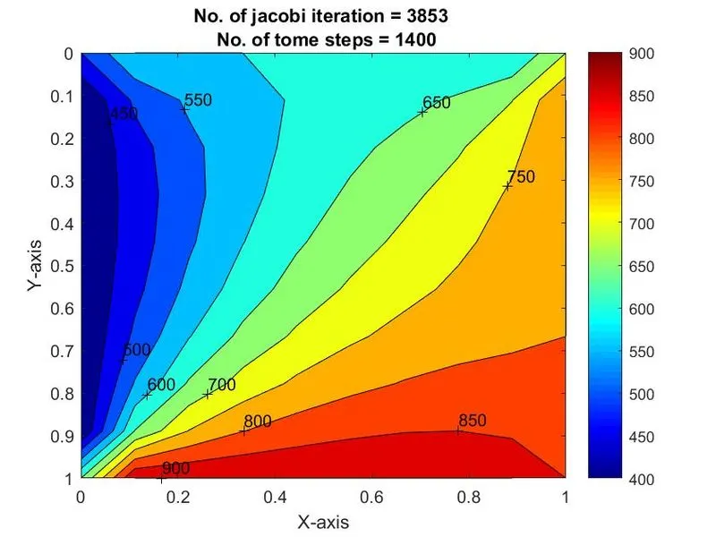
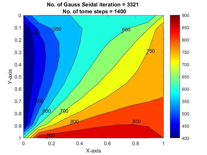
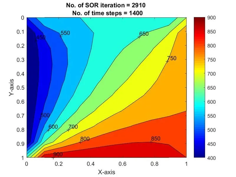
From the the above graphs it can be seen that the number of iteration required for jacobi is greater than gauss seidal and iteration for gauss seidal is greater than SOR. Thus we can say SOR can converge faster if proper relaxation parameter is considered.