Week 3.5 - Deriving 4th order approximation of a 2nd order derivative using Taylor Table method

1. Central Difernce Scheme : In CDS we will take same number of nodes on both the sides of node at which we want to find derivative. In this case we want to find differentiation at i th node.

Order of accuracy for CDS is given by ;

The order of accuracy P = Number of nodes in the stencil N - Order of derivative Q + 1

For our case P=4 (as we want 4th order accuracy) and Q=2

Therefore no of nodes we have to consider N = 4+2-1 ; N=5

`(∂^2 f)/(∂x^2 )=af(i-2)+bf(i-1)+cf(i)+df(i+1)+ef(i+2)`

Taylor table for CDS:

	f(x)	dx f’(x)	`dx^2 f''(x)`	`dx^3 f'''(x)`	`dx^4 f''''(x)`	`dx^5 f'''''(x)`	`dx^6 f''''''(x)`
af(i-2)	a	-2a	4a/2	-8a/6	16a/24	-32a/120	64a/240
bf(i-1)	b	-b	b/2	-b/6	b/24	-b/120	b/240
cf(i)	c	0	0	0	0	0	0
df(i+1)	d	d	d/2	d/6	d/24	d/120	d/240
ef(i+2)	e	2e	4e/2	8e/6	16e/24	32e/120	64e/240
af(i-2)+ bf(i-1)+ cf(i)+ df(i+1)+ ef(i+2)	0	0	1	0	0

Table can be written in matrix form as AX=B

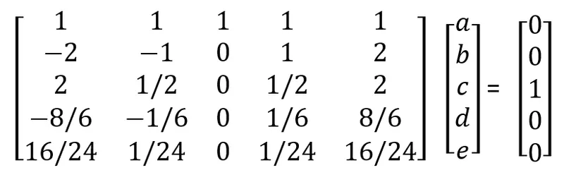
where X is coloum matrix having values of a,b,c,d and e.

After solving the above equation we get :

a=-0.0833
b=1.3333
c=-2.5000
d=1.3333
e=-0.0833

Now if we neglect 4th order and above terms we get

f''(x)= `(af(i-2)+bf(i-1)+cf(i)+df(i+1)+ef(i+2))/dx^2`

2. Skewed Right-Sided Difference : In this scheme we will take nodes on right side only.

Order of accuracy for CDS is given by ;

The order of accuracy P = Number of nodes in the stencil N - Order of derivative Q

For our case P=4 (as we want 4th order accuracy) and Q=2

Therefore no of nodes we have to consider N = 4+2 ; N=6

`(∂^2 f)/(∂x^2 )=af(i)+bf(i+1)+cf(i+2)+df(i+3)+ef(i+4)+ff(i+5)`

Taylor table for Skewed Right-Sided Difference:

	f(x)	dx f’(x)	`dx^2 f''(x)`	`dx^3 f'''(x)`	`dx^4 f''''(x)`	`dx^5 f'''''(x)`
af(i)	a	0	0	0	0	0
bf(i+1)	b	b	b/2	b/6	b/24	b/120
cf(i+2)	c	2c	4c/2	8c/6	16c/24	32c/120
df(i+3)	d	3d	9d/2	27d/6	81d/24	243d/120
ef(i+4)	e	4e	16e/2	64e/6	256e/24	1024e/120
ff(i+5)	f	5e	25e/2	125f/6	625f/24	3125f/120
af(i)+ bf(i+1)+ cf(i+2)+ df(i+3)+ ef(i+4)+ff(i+5)	0	0	1	0	0	0

As like central difference we can write this table also in matrix form and solve using matlab to get the coefficients as

a=3.7500
b=-12.8333
c=17.8333
d=-13.0000
e=5.0833
f=-0.8333

Now Similarly as CSD here we get

f''(x)=`(af(i)+bf(i+1)+cf(i+2)+df(i+3)+ef(i+4)+ff(i+5))/dx^2`

3.Skewed left-sided difference : In this scheme we will take nodes on left side only.

Order of accuracy for CDS is given by ;

The order of accuracy P = Number of nodes in the stencil N - Order of derivative Q

For our case P=4 (as we want 4th order accuracy) and Q=2

Therefore no of nodes we have to consider N = 4+2 ; N=6

`(∂^2 f)/(∂x^2 )=af(i-5)+bf(i-4)+cf(i-3)+df(i-2)+ef(i-1)+ff(i)`

Taylor table for Skewed Left-Sided Difference:

	f(x)	dxf’(x)	`dx^2f''(x)`	`dx^3f'''(x)`	`dx^4f''''(x)`	`dx^5f'''''(x)`
af(i-5)	a	-5a	25a/2	-125a/6	625a/24	-3125a/120
bf(i-4)	b	-4b	16b/2	-64b/6	256b/24	-1024b/120
cf(i-3)	c	-3c	9c/2	-27c/6	81c/24	-243c/120
df(i-2)	d	-2d	4d/2	-8d/6	16d/24	-32d/120
ef(i-1)	e	-e	e/2	-e/6	e/24	-e/120
ff(i)	f	0	0	0	0	0
af(i-5)+ bf(i-4)+ cf(i-3)+ df(i-2)+ef(i-1)+ff(i)	0	0	1	0	0	0

As like central difference and skewed left-sided differenceri we can write this table also in matrix form and solve using matlab to get the coefficients as

a=-0.8333
b=5.0833
c=-13.0000
d=17.8333
e=-12.8333
f=3.7500

After Neglecting 4th and higher order terms we get

f''(x)= `(af(i-5)+bf(i-4)+cf(i-3)+df(i-2)+ef(i-1)+ff(i))/dx^2`

Code for all the above matrix calculation and to plot graph for comparing the error for different approximations is given below

% Central Diffrencing Scheme
% solving matric equation  AX=B for Central Diffrencing Scheme
A= [1 1 1 1 1;-2 -1 0 1 2;2 0.5 0 0.5 2;-8/6 -1/6 0 1/6 8/6;16/24 1/24 0 1/24 16/24];
% we know X=[a;b;c;d;e];
B=[0;0;1;0;0];
% we have AX=B 
% to get x we have to do X= inverse(A)*B
X=inv(A)*B;

%Skewed Right-Sided Difference 
% Solving matric equation CY=D
C=[1 1 1 1 1 1;0 1 2 3 4 5 ;0 1/2 4/2 9/2 16/2 25/2;0 1/6 8/6 27/6 64/6 125/6;0 1/24 16/24 81/24 256/24 625/24;0 1/120 32/120 243/120 1024/120 3125/120];
D=[0;0;1;0;0;0];
% to get Y we have to do Y= inverse(C)*D
Y=inv(C)*D;

%Skewed Left-Sided Difference 
% Solving matric equation EZ=F
E=[1 1 1 1 1 1;-5 -4 -3 -2 -1 0 ;25/2 16/2 9/2 4/2 1/2 0;-125/6 -64/6 -27/6 -8/6 -1/6 0;625/24 256/24 81/24 16/24 1/24 0;-3125/120 -1024/120 -243/120 -32/120 -1/120 0];
F=[0;0;1;0;0;0];
% to get Z we have to do Z= inverse(E)*F
Z=inv(E)*F;

% Now calculating derivative using Analytical,CDS,SRSD and SLSD
% given function is f(x)=exp(x)*cos(x)
 % Anallytical Derivative f''(x)=-2*exp(x)*sin(x)
 x=pi/3;
 dx=linspace(pi/40,pi/4000,20);
 f=@(x)(exp(x)*cos(x));
 Analytical_Derivative=-2*exp(x)*sin(x)
  % Using Numerical schemes
  CDS=zeros(1,20);
  SRSD=zeros(1,20);
 SLSD=zeros(1,20);
 for i=1:20
 % Using CDS
 % f''(x)=af(i-2)+bf(i-1)+cf(i)+df(i+1)+ef(i+2)
 % X=[a;b;c;d;e] i.e. its a coloumn matrix.
 CDS(i)=(X(1)*f(x-2*dx(i))+X(2)*f(x-dx(i))+X(3)*f(x)+X(4)*f(x+dx(i))+X(5)*f(x+2*dx(i)))/dx(i)^2;
 CDS_error(i)=abs(Analytical_Derivative-CDS(i));
 
 % Using SRSD
 % f''(x)=af(i)+bf(i+1)+cf(i+2)+df(i+3)+ef(i+4)+ff(i+5)
 % Y=[a;b;c;d;e;f] i.e. its a coloumn matrix.
 SRSD(i)=(Y(1)*f(x)+Y(2)*f(x+dx(i))+Y(3)*f(x+2*dx(i))+Y(4)*f(x+3*dx(i))+Y(5)*f(x+4*dx(i))+Y(6)*f(x+5*dx(i)))/dx(i)^2;
 SRSD_error(i)=abs(Analytical_Derivative-SRSD(i));
 
 % Using SLSD
 % f''(x)=af(i-5)+bf(i-4)+cf(i-3)+df(i-2)+ef(i-1)+ff(i)
 % Y=[a;b;c;d;e;f] i.e. its a coloumn matrix.
 SLSD(i)=(Z(1)*f(x-5*dx(i))+Z(2)*f(x-4*dx(i))+Z(3)*f(x-3*dx(i))+Z(4)*f(x-2*dx(i))+Z(5)*f(x-dx(i))+Z(6)*f(x))/dx(i)^2;
 SLSD_error(i)=abs(Analytical_Derivative-SLSD(i));
 end
 % Now plotting graphs to compare error for CDS,SRSD and SLSD at diffrent dx
plot(dx,CDS_error);
hold on
plot(dx,SRSD_error,'r');
hold on
plot(dx,SLSD_error,'g');
legend('CSD orror','SRSD error','SLSD error')
xlabel('Grid size (dx)');
ylabel('Error');
title('Error Vs Grid size(dx)');

Result :

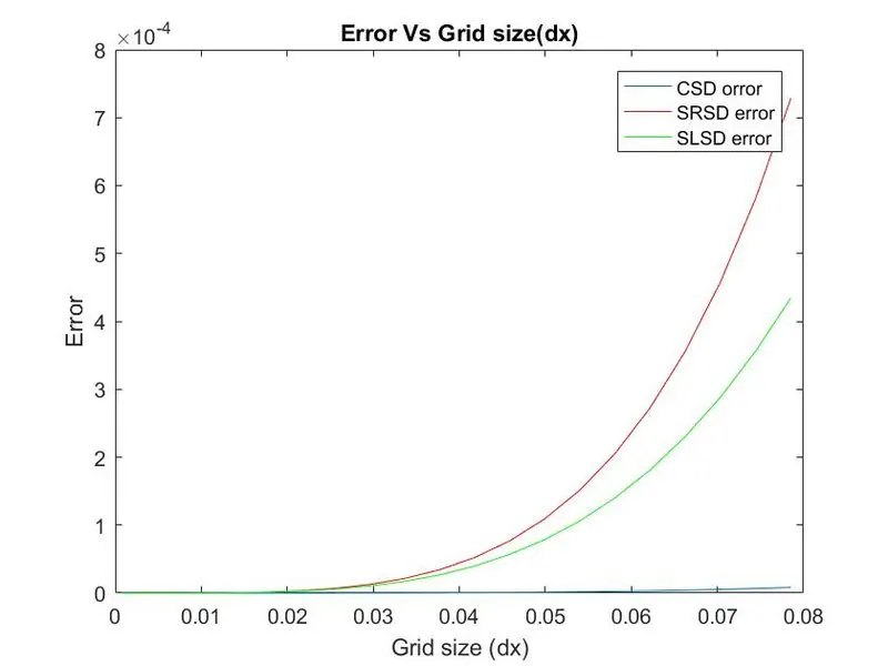
1. From the above grapth it can be seen that as grid size decreases error goes on decreasing anf finally becomes nearly zero.

2. Error for CDS is always less than right and left skewed scheme.

3. Error for CDS quickly reduces to zero as compare to right and left skewed scheme

why a skewed scheme is useful:

When we know the value at end point of domain we can only use skewed scheme there we cant use central difference scheme to find the values at other nodes.

For example if we know the value of temperature at one end of wall we have to use forward scheme only to find values of tempeerature inside and at other end of wall.

But CDS is more accurate and gives faster results.