Week 7 - Simulation of a 1D Super-sonic nozzle flow simulation using Macormack Method
The subsonic-supersonic nozzle is a general type of converging-diverging nozzle which are majorly used to provide enough thrust force utilized from its high velocities at the end portion of the nozzle which is desired to be of a supersonic kind. Here, for simulation of this type of nozzle, we consider a steady, isentropic flow through it and, even though when the area of the nozzle when considered which represents a 2-dimensional space, we consider the flow only along the length of the nozzle, i.e., 1-dimensional flow through the duct which is more similar to the results which we get from the 2-dimensional analysis wherein the later is the hardest way to the solution. Thus such a flow is said to be a Quasi-One dimensional flow. The below is the image shown for the isentropic flow condition through the subsonic-supersonic nozzle.
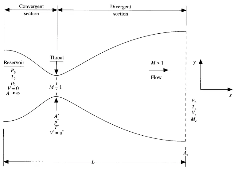
The analytical way of solving the solution for the flow through the converging-diverging nozzle can be represented from the equations as a function of the Mach number, which is represented as follows,

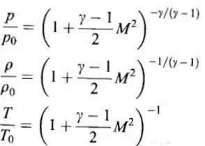
Source: Computational fluid dynamics: the basics with applications by John Anderson
Where the above equations represent the variation of pressure, density, and temperature as a function of Mach number along the length of the nozzle.
The flow doesn't happen just by itself but must have a suitable pressure difference between its ends such that the flow occurs through the duct to meet the necessary purpose for this type of nozzle.
GOVERNING FLOW EQUATIONS:
The numerical analysis done to obtain the solutions is taken care of by the Governing equations. The governing equations are couched in formats of the partial differential equations making them suitable for time-marching solutions for the considered Quasi 1-dimensional nozzle flow.
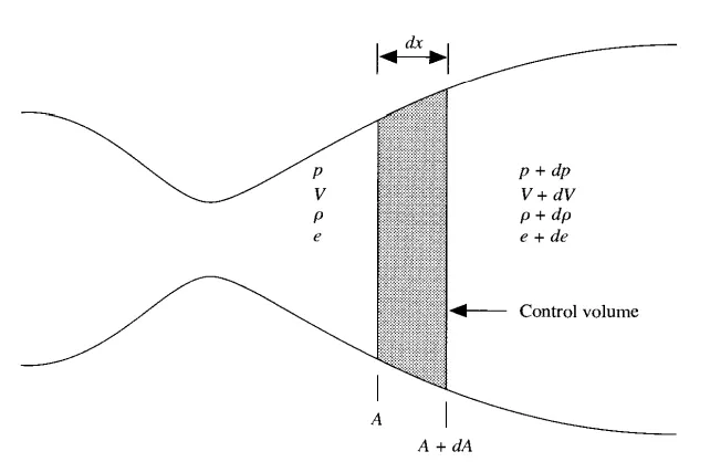
The equations that are likely to be appropriate for the Quasi 1 dimensional flow can be assumed as, the 1) Mass conservation equation, 2) Momentum conservation equation, and 3) Energy conservation equation, for which we apply the integral forms of these equations into a control volume. Here we basically have a control volume and write those above equations in terms of the integral quantities over the control volume.
WHAT IS NON-CONSERVATIVE AND CONSERVATIVE FORM AND WHAT IS THE DIFFERENCE BETWEEN THEM?
In general, when we are looking at the numerical solution for a given problem, we would say that the results are correct unless and until when we realize that the analytical solutions give better results in comparison to the numerical solution results. But, we do have some classification within the numerical analysis based on the modification of the governing equations solely for the purpose of attaining better results from one over the other, and this classification is 1) Non-Conservative, and the 2) Conservative form.
Both these forms are not entirely different based on the structure of their governing equations but one can be derived from the other with a simple expansion process, while the Non-Conservative form has only the primitive variables(density, velocity, temperature) and the Conservative form has the flux of the primitive variables inside the divergence operator.
The differences between the two forms can be said that
- The Non-conservative form makes use of the Lagrangian approach while the Conservative form makes use of the Eulerian approach.
- Based on the convenience for coding we can say that the primitive variables can be solved directly in the Non-conservative form and hence is easier for coding while the primitive variables can only be obtained from the indicated flux terms in the Conservative form which eventually makes the programing difficult.
- In terms of accuracy, we know that the increased number of calculation steps makes the system round off the solution results due to machine precision, and thus we know that the Non-conservative form directly deals with the primitive variables while the conservative form deals indirectly through the flux terms, which makes the Conservative form give a more accurate result.
- In terms of Convergence rate, since the Non-conservative form has direct primitive variable calculating measures, we may have a quicker converged solution result for it in comparison to the Conservative form which indirectly deals through the fluxes.
- The main conceptual difference comes into play only when considering the Stability criterion for both forms. In general, the numerical solution method deals with partial differential equations which may sometimes lead to discontinuities of the solution, and this phenomenon when applied to the above two forms, we may still have discontinuities while going with the Non-Conservative form since it deals with the direct primitive variables, while having a perfect run without any blow ups or discontinuities for the Conservative form. This is the main purpose why many engineering problems make use of the Conservative form of Governing equations.
1) Continuity equation:
The surface and volume integrals for the continuity equation and their respective relations are given as,
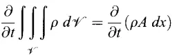 is the volume integral for the Rate of change of mass inside a control volume(dV).
 is the surface integral for the Rate of change of mass inside a control volume(dS).
The relation between them is given as,
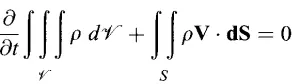
And hence, when we expand the terms and substitute, we end up with the Governing equation for the Continuity equation which is expressed as follows,
Conservative Form:
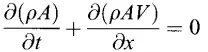
Non-Conservative Form:
[∂(ρA) + v∂( ρA)/ ∂x ] = - ρA(∂v/ ∂x)
Also, we represent the above forms of governing equations in the form of Non-dimensional quantities of the primitive variables which are given by,
 ;
; ;
; ;
;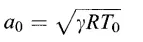 ;
; ;
;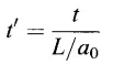 ;
;
Non-dimensional form of Non-Conservative form:

Non-dimensional form of Conservative form:
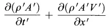 = 0
= 0
2) Momentum conservation equation:
The surface and volume integrals over a control volume(dV) and over the surface(dS or area vector) for the momentum equation is given as,
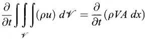

And the relation between them is,

Depending on the direction of the area vector, over the control volume, as seen in the above figure, which affects the evaluation of the pressure term on the right-hand side, we fix some force vectors for the ease of calculation of the pressure term, which is represented in the below figure.
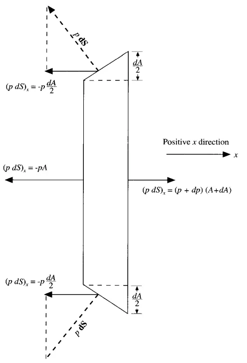
And at last, we end up with the Governing equation for the x-Momentum equation which is expressed as follows,
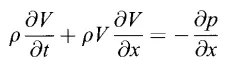
Conservative form:
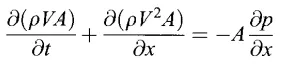
Non-Conservative form:
Non-dimensional form of Non-Conservative form:

Non-dimensional form of Conservative form:

3) Energy conservation equation:
As seen from the above equations, similar is the case for the energy conservation equation, and the relation is expressed as,

And hence, when we expand the terms and substitute, we end up with the Governing equation for the Energy conservation equation which is expressed as follows,
Conservative form:

Non-Conservative form:

Non-dimensional form of Non-Conservative form:

Non-dimensional form of Conservative form:

Note: For Conservative forms of Governing equations, we separate the equation into 3 types of vector terms, that is,
- Solution Vector
- Flux Vector
- Source Term
Where, from the Conservative forms of Continuity, Momentum, and Energy equations, we can separate and write the above vector form for it.
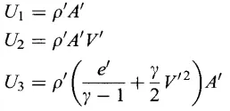 are the solution vectors, separated from the above Conservative Governing equations.
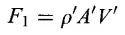
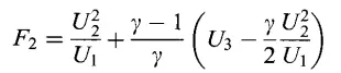
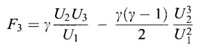 are the Flux vectors, separated from the above Conservative Governing equations.
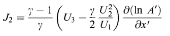 is the Source term, separated from the above Conservative Governing equations.
CFD SOLUTION USING MACCORMACK'S METHOD:
In general, till now, we learned and followed a method called the Lax-Wandroff Technique, which represents the function in terms of the Taylor series expansion with having the accuracy in the order of time(dt). But here, we use a new method called MacCormack's method, so that the algebra is solved in a way without bringing in the calculation of 2nd order time-derivative but only by taking the average values of the time-derivative of the primitive variables.
The average values of the time-derivative term are calculated from two steps,
- Predictor Step
- Corrector step
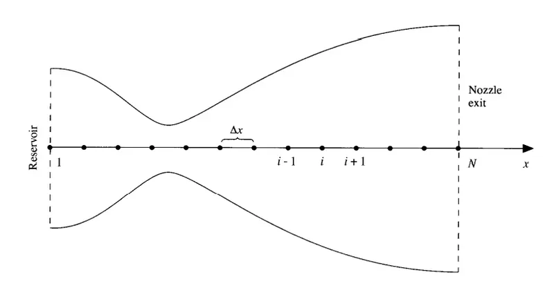
Note: For explanation let us take the example of the Continuity equation for the Non-conservative form in a subsonic-supersonic nozzle. Below is the image given, representing the grid point distribution along the nozzle.
Non-Conservative form:
1) Predictor step:
In this step, we apply a forward differencing scheme for the spatial derivatives terms in the respective governing equation(here, Continuity equation), for the same time-step employed in both spatial and time derivative terms on the R.H.S and L.H.S of the equation.
The Forward differencing scheme applied to the non-conservative form of continuity equation from the above is given as,

Now analogous to the following equations the above calculated time-derivative terms are substituted, thus forming the values of the primitive variables at a new time step.
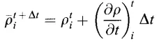 Here, the first term of the R.H.S is a known value taken from the initial boundary conditions, and the second term values are taken from the previous step of the calculation.
Calculation of the time-step:
In accordance with the CFL condition, wherein the time difference term(dt), can be represented as,
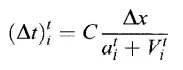
And it seems like the dt values change for every grid point due to the change in the velocity of the flow inside the duct. Although the dt values can be calculated from the local time-marching solutions, the solutions feel to be providing a slight discomfort in terms of the stability of the solution, and hence we consider the minimum value of time(dt) for a given single time-step and thus leading to a perfectly stable result.

2) Corrector step:
In this step, we apply a rearward differencing scheme for the spatial derivative terms of the governing equation, for the same time-step employed in both spatial and time derivative terms on the R.H.S and L.H.S of the equation.
The Rearward differencing scheme applied to the non-conservative form of continuity equation from the above is given as,
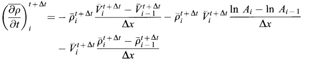
Now analogous to the following equations the above calculated time-derivative terms from both the steps are consolidated to form the average of the time-derivative terms.
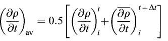
Now, finally, the above solutions can be solved employed at the following equation, to come up with the new value of the primitive variable at the new time step.
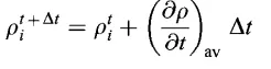
Thus the same procedure is employed for the momentum and energy equation to come up with the values of the velocity and temperature at their new time steps.
Conservative form:
The conservative form also will be solved in the same manner under the MacCormack method as the Non-Conservative part, but the only difference is that, since the Conservative part deals with the primitive variables in an indirect way, we will do all the above similar procedures for the Flux vector(F) to solve for the Solution vector(U), which are represented initially with the equations as,
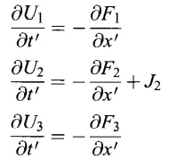
From here, in a very similar way to what we saw in the non-conservative form, in the predictor step, the Fluxvectors are forward differenced and the solution vectors are updated with its values for the next time-step and then finding the average of the solution vectors to end up with the finding of the values of the Primitive variables.
BOUNDARY CONDITIONS:
Boundary conditions are very essential, that is, without which a proper numerical result cannot be obtained. In our case, the inlet boundary is represented at the start of the converging nozzle, and the outlet boundary conditions are represented at the end of the diverging section of the nozzle. Here even though the 1st point(inlet) is present in the reservoir, its velocity is taken to be a non zero and closer value to zero. This is because the theoretical value tends only to be zero, but practically we have to apply a certain velocity more than zero to cause the flow to happen even when it has an area cross-section of infinite(here area of the reservoir is taken).
We also know that this case follows an unsteady inviscid flow that eventually reaches the steady-state at a due point of time and thus such type of flow is governed by hyperbolic equations, wherein there exist two real characteristic lines at any point in the xt plane.
For our case, the xt plane can be shown as,
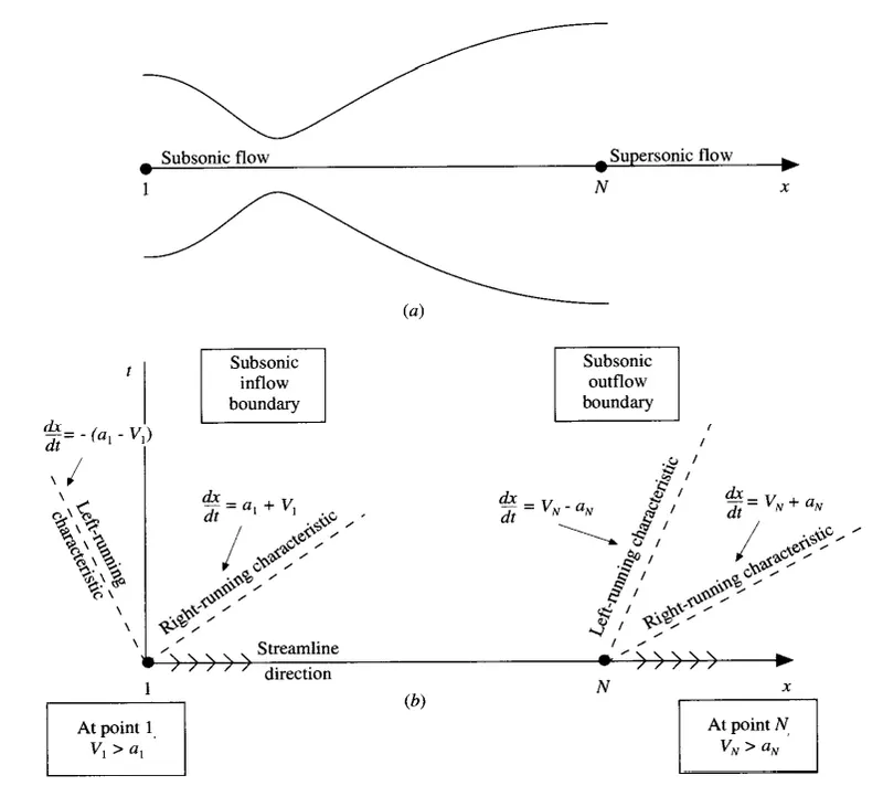
From the above image, we can make a corresponding conclusion that, at the inlet point where we'll be having 2 characteristic lines and here, one of them is traveling away from the streamline direction and another one is traveling inside the duct following the streamline direction. Thus the Left-running characteristic line must be allowed to float and that characteristic line is assumed to be a characteristic variable assigned as velocity, on the physical basis of allowing the mass flow to adjust itself to a steady-state, and thus it makes sense for the selection of velocity as the floating variable. Whereas, the other two variables, that is, Density and Temperature, are assigned values equal to 1.
Similarly, at the outlet boundary condition, both the characteristic lines run outside the domain and we comfortably say that all the three characteristic variables must be allowed to float, thus assuming a simple linear equation with the help of the neighboring values.
For the Non-Conservative form, we have the following set of boundary conditions,
Subsonic Inflow Boundary(Point 1):
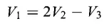 , obtained from linear extrapolation.
 where these are fixed and independent of time.
Supersonic Inflow Boundary(Point n):
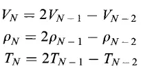 , obtained from linear extrapolation.
For the Conservative form, we have the following set of boundary conditions,
Subsonic Inflow Boundary(Point 1):
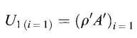
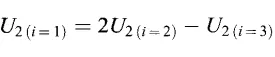
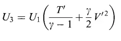
Supersonic Inflow Boundary(Point n):
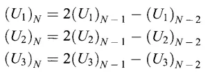
INITIAL CONDITIONS:
The inlet conditions must choose a bit carefully because, the farther the inlet conditions are from the solution, the greater is the time needed to converge to the solution, and also more initial unstableness tending to push the solution to attain the stable condition.
Thus at time t=0, the initial conditions for the non-conservative form are given as,
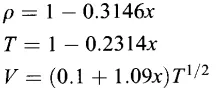
At time t=0, the initial conditions for the non-conservative form are given as,

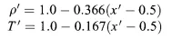

Area of the nozzle: The area of the nozzle is held fixed irrespective of the variation with the time, and is in general represented as,

Let us perform the analysis of the 1-dimensional flow through the subsonic-supersonic nozzle through MATLAB and also find out the output results of the primitive variables for both Conservative and Non-Conservative forms, and also will perform a Grid independence test.
MAIN CODE:
The main CODE comprising the functions for Conservative and Non-Conservative form, and other functions related to the graph plots, is given below.
clear all
close all
clc
n=[31 61 91];                                                              %nodes required for grid independance test
for i = 1: length(n)                                                       %Nodal loop
    input.i=i;
    input.length_n=length(n);                                              %total number of nodes required for grid independance test
    input.n=n(i);                                                          %number of nodes
    input.x=linspace(0,3,input.n);                                         %length of the nozzle
    input.dx=input.x(2)-input.x(1);                                        %dx value

    %%
    %outer loop
    input.sp_ht=1.4;                                                       %specific heat ratio
    input.nt=1400;                                                         %no. of time steps
    input.length_nt=linspace(1,input.nt,input.nt);                         %length of time step as per graph
    input.time_step=0;

    %calling the function for Non-Conservative form:
    [output_nc]= non_cons_nozzle_fresh(input)

    %calling the function for Conservative form:
    [output_c] = cons_nozzle_fresh(input)

    %defining seperate inputs for given number of nodes
    if i==1
        input_1=input;
    elseif i==2
        input_2=input;
    elseif i==3
        input_3=input;
    end


    %defining seperate outputs for given number of nodes(NON-CONSERVATIVE FORM)
    if i==1
        output_nc_1=output_nc;
    elseif i==2
        output_nc_2=output_nc;
    elseif i==3
        output_nc_3=output_nc;
    end


    %defining seperate outputs for given number of nodes(CONSERVATIVE FORM)
    if i==1
        output_c_1=output_c;
    elseif i==2
        output_c_2=output_c;
    elseif i==3
        output_c_3=output_c;
    end

end
    %Comparison plots made between the Conservative and Non-Conservative forms:
    plot_compare(input_1,input_2,input_3,output_c_1,output_nc_1,output_c_2,output_nc_2,output_c_3,output_nc_3)

    %Grid independance test using bar plots
    br_plots(input,output_c_1,output_nc_1,output_c_2,output_nc_2,output_c_3,output_nc_3)
Here, the necessary inputs and required outputs are just inherited and taken out just by using the keywords as a function followed by a dot(.), that is, input. , output.
Now we call upon the function for Non-Conservative form, and it is given below.
function [output]= non_cons_nozzle_fresh(input)
x=input.x;
dx=input.dx;
n=input.n;
nt=input.nt;
time_step=input.time_step;
sp_ht=input.sp_ht;
node_num=input.i;

%initial condition:
rho = 1- (0.3146.*x) ;                                                     %density
t = 1- (0.2314.*x);                                                        %temperature
v = (0.1 + 1.09.*x).*(t).^0.5;                                             %velocity
a=1+(2.2.*(x-1.5).^2);                                                     %area(parabolic)
n_th=find(a==1);
%%
%time step:
C=0.5;                                                                     %courant number based time steep control:
%Aim=To find minumum value of time step of all the grid points:
for k=1:length(x)
    a_vel(k)=(t(k)).^0.5;
    dt_eg(k)= C*dx/(a_vel(k) + v(k));
end
dt=min(dt_eg);                                                             %finding the minimum of dt with respect to C.
%%
for i=1:nt
    %old values
    rho_old=rho;
    v_old=v;
    t_old=t;
    for j=2:(n-1)
        %predictor step
        dvdx= (v(j+1)-v(j))/dx;
        dtdx= (t(j+1)-t(j))/dx;
        drhodx= (rho(j+1)-rho(j))/dx;
        dlogadx= (log(a(j+1))-log(a(j)))/dx;

        %continuity equation
        drhodt_p(j)= -(rho(j)*dvdx)-(rho(j)*v(j)*dlogadx)- (v(j)*drhodx);

        %momentum equation
        dvdt_p(j)= -(v(j)*dvdx)-(1/sp_ht)*(dtdx+ (t(j)/rho(j))*drhodx);

        %enery equation
        dtdt_p(j)= -(v(j)*dtdx)-(sp_ht-1)*t(j)*(dvdx + v(j)*dlogadx);

        %solution
        rho(j)= rho(j)+drhodt_p(j)*dt;
        v(j)=v(j)+dvdt_p(j)*dt;
        t(j)=t(j)+dtdt_p(j)*dt;
    end

    for u=2:(n-1)
        %corrector step
        dvdx = (v(u)-v(u-1))/dx;
        dtdx= (t(u)-t(u-1))/dx;
        drhodx= (rho(u)-rho(u-1))/dx;
        dlogadx= (log(a(u))-log(a(u-1)))/dx;

        %continuity equation
        drhodt_c(u)= -(rho(u)*dvdx)-(rho(u)*v(u)*dlogadx)- (v(u)*drhodx);

        %momentum equation
        dvdt_c(u)= -(v(u)*dvdx)-(1/sp_ht)*(dtdx+ (t(u)/rho(u))*drhodx);

        %enery equation
        dtdt_c(u)= -(v(u)*dtdx)-(sp_ht-1)*t(u)*(dvdx + v(u)*dlogadx);
    end

    %computing the solution:
        drhodt_avg=0.5*(drhodt_p + drhodt_c);
        dvdt_avg=0.5*(dvdt_p + dvdt_c);
        dtdt_avg=0.5*(dtdt_p + dtdt_c);


    %solution
    for m=2:(n-1)
    rho(m) = rho_old(m) + drhodt_avg(m)*dt;
    v(m) = v_old(m) + dvdt_avg(m)*dt;
    t(m) = t_old(m) + dtdt_avg(m)*dt;

    end
 %%
    %Boundary conditions
    %inlet
    v(1)=2*v(2)-v(3);                                                      %floating variable
    rho(1)=1;
    t(1)=1;

    %outlet
    v(n)= 2*v(n-1)-v(n-2);                                                 %floating variable
    rho(n)= 2*rho(n-1)-rho(n-2);                                           %floating variable
    t(n)= 2*t(n-1)-t(n-2);                                                 %floating variable

    output.v = v;                                                          %velocity
    output.rho = rho;                                                      %density
    output.t = t;                                                          %temperature
    output.p= rho.*t;                                                      %pressure
    output.m= v./(t).^0.5;                                                 %mach number
    output.mfr= rho.*a.*v;                                                 %mass flow rate
    output.mfr_th= rho.*(t).^0.5;                                          %mass flow rate at throat(non-dimensional form)
%%
    %flow field variables in throat
    output.rho_th(i) = output.rho(n_th);
    output.v_th(i) = output.v(n_th);
    output.t_th(i) = output.t(n_th);
    output.p_th(i) = output.p(n_th);
    output.m_th(i) = output.m(n_th);
    output.MFR_th(i) = output.mfr_th(n_th);


    %Plotting mass flow rate for various time steps
    i_terms=[1 50 100 150 200 700 1400];
    for g=1:length(i_terms)
        if i==i_terms(g)
        figure(node_num)
        plot(x,output.mfr)
        no_of_nodes= n;
        txt=[' Variation of Mass flow Rate as a function of distance over increasing time steps with number of nodes = ',int2str(no_of_nodes)]
        title(txt)
        subtitle('Non-Conservative form')
        legend('Initial condition','50t time step','100t time step','150t time step','200t time step','700t time step','1400th time step')
        ylabel('Mass flow Rate')
        xlabel('Non-dimensional distance through the nozzle(x)')
        grid on
        hold on
        end

    end
    time_step= time_step+1;
end
    output.mfr_final_nc= output.mfr;
end
Now we call upon the function for Conservative form, and it is given below.
function [output]=cons_nozzle_fresh(input)
%initial condition:
x=input.x;
dx=input.dx;
n=input.n;
nt=input.nt;
node_num=input.i;
length_n=input.length_n;
a=1+(2.2.*(x-1.5).^2);                                                     %nozzle area
n_th=find(a==1);

for i=1:n
    if x(i)>=0 && x(i)<=0.5
        rho(i)=1;
        t(i)=1;

    elseif x(i)>=0.5 && x(i)<=1.5
        rho(i)=1-0.366*(x(i)-0.5);
        t(i)=1-0.167*(x(i)-0.5);

    else x(i)>=1.5 && x(i)<=3.5
    rho(i)=0.634-0.3879*(x(i)-1.5);
    t(i)=0.833-0.3507*(x(i)-1.5);

    end
end
v=0.59./(rho.*a);
p= rho.* t;
%%
%CONSERVATIVE FORM:
%time step:
C=0.5;                                                                     %courant number based time steep control:
%Aim=To find minumum value of time step of all the grid points:
for m=1:length(x)
    a_vel(m)=(t(m)).^0.5;
    dt_eg(m)= C*dx/(a_vel(m) + v(m));
end
dt=min(dt_eg);

sp_ht = 1.4;                                                               %specific heat ratio
%setting the values of U(solution vectors) to optimise F(flux vectors):
u1=rho.*a;
u2=rho.*a.*v;
u3=rho.*a.*((t./(sp_ht-1))+((sp_ht/2).*(v).^2));


time_step= 1;
%length_nt=linspace(1,nt,nt);
for k=1:nt
    u1_old=u1;
    u2_old=u2;
    u3_old=u3;

    f1=u2;
    f2=(((u2).^2)./u1) + ((sp_ht-1)/sp_ht).*(u3-(sp_ht/2).*(((u2).^2)./u1));
    f3=((sp_ht.*u2.*u3)./u1) - ((sp_ht*(sp_ht-1)/2).*(((u2).^3)./(u1).^2));

    %Predictor step
    for j=2:(n-1)
        dfdx_1(j)= (f1(j+1)- f1(j))/dx;
        dfdx_2(j)= (f2(j+1)- f2(j))/dx;
        dfdx_3(j)= (f3(j+1)- f3(j))/dx;
        j2(j)    = ((1/sp_ht)*rho(j)*t(j)*(a(j+1)-a(j))/dx);

        dudt_1_p(j)= -(dfdx_1(j));
        dudt_2_p(j)= -(dfdx_2(j))+j2(j);
        dudt_3_p(j)= -(dfdx_3(j));

        u1(j) = u1(j) + (dudt_1_p(j))*dt;
        u2(j) = u2(j) + (dudt_2_p(j))*dt;
        u3(j) = u3(j) + (dudt_3_p(j))*dt;

    end
    %updating the primitive variables
    rho = u1./a;                                                           %density
    v   = u2./u1;                                                          %velocity
    t   =(sp_ht-1).*((u3./u1)-(0.5*sp_ht.*v.^2));                          %temperature
    p   = rho.*t;                                                          %pressure

    %updating the flux terms
    f1=u2;
    f2=(((u2).^2)./u1) + ((sp_ht-1)/sp_ht).*(u3-(sp_ht/2).*(((u2).^2)./u1));
    f3=((sp_ht.*u2.*u3)./u1) - ((sp_ht*(sp_ht-1)/2).*(((u2).^3)./(u1).^2));

    %Corrector step
    for y=2:(n-1)
        dfdx_1(y)= (f1(y) - f1(y-1))/dx;
        dfdx_2(y)= (f2(y) - f2(y-1))/dx;
        dfdx_3(y)= (f3(y) - f3(y-1))/dx;
        j2(y)    = ((1/sp_ht)*rho(y)*t(y)*(a(y)-a(y-1))/dx);

        dudt_1_c(y)= -(dfdx_1(y));
        dudt_2_c(y)= -(dfdx_2(y))+j2(y);
        dudt_3_c(y)= -(dfdx_3(y));

    end

    dudt_1_avg = 0.5 * (dudt_1_p + dudt_1_c);
    dudt_2_avg = 0.5 * (dudt_2_p + dudt_2_c);
    dudt_3_avg = 0.5 * (dudt_3_p + dudt_3_c);

    for h=2:(n-1)
        u1(h)= u1_old(h) + (dudt_1_avg(h))*dt;
        u2(h)= u2_old(h) + (dudt_2_avg(h))*dt;
        u3(h)= u3_old(h) + (dudt_3_avg(h))*dt;
    end
%%
    %Boundary conditions
    %inlet
    u1(1)=rho(1)*a(1);
    u2(1)=(2*u2(2))-u2(3);
    v(1)=u2(1)/u1(1);
    u3(1)=u1(1) * ((t(1)/(sp_ht-1)) + ((sp_ht/2)*v(1)^2));

    %outlet
    u1(n)= 2*u1(n-1)-u1(n-2);
    u2(n)= 2*u2(n-1)-u2(n-2);
    u3(n)= 2*u3(n-1)-u3(n-2);

    %updating the primitive flow field variables
    output.u1=u1;
    output.u2=u2;
    output.u3=u3;
    output.rho = u1./a;                                                    %density
    output.v   = u2./u1;                                                   %velocity
    output.t   =(sp_ht-1).*((u3./u1)-(0.5*sp_ht.*v.^2));                   %temperature
    output.p   = rho.*t;                                                   %pressure
    output.m= v./(t).^0.5;                                                 %mach number
    output.mfr= rho.*a.*v;                                                 %mass flow rate
    output.mfr_th= rho.*(t).^0.5;                                          %mass flow rate at throat(non-dimensional form)

    %Primitive variables at the throat
    output.rho_th(k) = output.rho(n_th);
    output.v_th(k) = output.v(n_th);
    output.t_th(k) = output.t(n_th);
    output.p_th(k) = output.p(n_th);
    output.m_th(k) = output.m(n_th);
    output.MFR_th(k) = output.mfr_th(n_th)


    %Plotting mass flow rate for various time steps
    k_terms=[1 50 100 150 200 700 1400];
    for g=1:length(k_terms)
        if k==k_terms(g)
        figure(node_num+length_n)
        plot(x,output.mfr)
        no_of_nodes= n;
        txt=[' Variation of Mass flow Rate as a function of distance over increasing time steps with number of nodes = ',int2str(no_of_nodes)]
        title(txt)
        subtitle('Conservative form')
        legend('Initial condition','50t time step','100t time step','150t time step','200t time step','700t time step','1400th time step')
        ylabel('Mass flow Rate')
        xlabel('Non-dimensional distance through the nozzle(x)')
        grid on
        hold on
        end
    end

    time_step = time_step +1;
end
    output.mfr_final_c= output.mfr;
end
Now we call upon the function made for the comparison of primitive variables and their change based on the number of nodes, time steps, length of the nozzle, etc, and it is given below.
function plot_compare(input_1,input_2,input_3,output_c_1,output_nc_1,output_c_2,output_nc_2,output_c_3,output_nc_3)

     x_1=input_1.x;
     length_nt_1=input_1.length_nt;

     figure(7)
     subplot(5,1,1)
     plot(x_1,output_nc_1.v)
     hold on
     plot(x_1,output_c_1.v,'*')
     grid on
     legend('Non-Conservtive','Conservative')
     title('Velocity variation along the length of the nozzle for n=31')
     xlabel('Length of the nozzle')
     ylabel('Velocity')


     subplot(5,1,2)
     plot(x_1,output_nc_1.rho)
     hold on
     plot(x_1,output_c_1.rho,'*')
     grid on
     legend('Non-Conservtive','Conservative')
     title('Density variation along the length of the nozzle for n=31')
     xlabel('Length of the nozzle')
     ylabel('Density')


     subplot(5,1,3)
     plot(x_1,output_nc_1.t)
     hold on
     plot(x_1,output_c_1.t,'*')
     grid on
     legend('Non-Conservtive','Conservative')
     title('Temperature variation along the length of the nozzle for n=31')
     xlabel('Length of the nozzle')
     ylabel('Temperature')


     subplot(5,1,4)
     plot(x_1,output_nc_1.p)
     hold on
     plot(x_1,output_c_1.p,'*')
     grid on
     legend('Non-Conservtive','Conservative')
     title('Pressure variation along the length of the nozzle for n=31')
     xlabel('Length of the nozzle')
     ylabel('Presuure')

     subplot(5,1,5)
     plot(x_1,output_nc_1.m)
     hold on
     plot(x_1,output_c_1.m,'*')
     grid on
     legend('Non-Conservtive','Conservative')
     title('Mach number variation along the length of the nozzle for n=31')
     xlabel('Length of the nozzle')
     ylabel('Ma')

     %%
     figure(8)
     subplot(6,1,1)
     plot(length_nt_1,output_nc_1.v_th)
     hold on
     plot(length_nt_1,output_c_1.v_th)
     grid on
     legend('Non-Conservtive','Conservative')
     title('Variation of Velocity at the throat w.r.t number of Time-steps for n=31')
     xlabel('Time steps')
     ylabel('Velocity')


     subplot(6,1,2)
     plot(length_nt_1,output_nc_1.rho_th)
     hold on
     plot(length_nt_1,output_c_1.rho_th)
     grid on
     legend('Non-Conservtive','Conservative')
     title('Variation of Density at the throat w.r.t number of Time-steps for n=31')
     xlabel('Time steps')
     ylabel('Density')


     subplot(6,1,3)
     plot(length_nt_1,output_nc_1.t_th)
     hold on
     plot(length_nt_1,output_c_1.t_th)
     grid on
     legend('Non-Conservtive','Conservative')
     title('Variation of Temperature at the throat w.r.t number of Time-steps for n=31')
     xlabel('Time steps')
     ylabel('Temperature')


     subplot(6,1,4)
     plot(length_nt_1,output_nc_1.p_th)
     hold on
     plot(length_nt_1,output_c_1.p_th)
     grid on
     legend('Non-Conservtive','Conservative')
     title('Variation of Pressure at the throat w.r.t number of Time-steps for n=31')
     xlabel('Time steps')
     ylabel('Presuure')

     subplot(6,1,5)
     plot(length_nt_1,output_nc_1.m_th)
     hold on
     plot(length_nt_1,output_c_1.m_th)
     grid on
     legend('Non-Conservtive','Conservative')
     title('Variation of Mach number at the throat w.r.t number of Time-steps for n=31')
     xlabel('Time steps')
     ylabel('Ma')

     subplot(6,1,6)
     plot(length_nt_1,output_nc_1.MFR_th)
     hold on
     plot(length_nt_1,output_c_1.MFR_th)
     grid on
     legend('Non-Conservtive','Conservative')
     title('Variation of Mass Flow Rate at the throat w.r.t number of Time-steps for n=31')
     xlabel('Time steps')
     ylabel('Ma')

    %%
    x_2=input_2.x;
    length_nt_2=input_2.length_nt;


    figure(9)
    subplot(5,1,1)
    plot(x_2,output_nc_2.v)
    hold on
    plot(x_2,output_c_2.v,'*')
    grid on
    legend('Non-Conservtive','Conservative')
    title('Velocity variation along the length of the nozzle for n=61')
    xlabel('Length of the nozzle')
    ylabel('Velocity')


    subplot(5,1,2)
    plot(x_2,output_nc_2.rho)
    hold on
    plot(x_2,output_c_2.rho,'*')
    grid on
    legend('Non-Conservtive','Conservative')
    title('Density variation along the length of the nozzle for n=61')
    xlabel('Length of the nozzle')
    ylabel('Density')


    subplot(5,1,3)
    plot(x_2,output_nc_2.t)
    hold on
    plot(x_2,output_c_2.t,'*')
    grid on
    legend('Non-Conservtive','Conservative')
    title('Temperature variation along the length of the nozzle for n=61')
    xlabel('Length of the nozzle')
    ylabel('Temperature')


    subplot(5,1,4)
    plot(x_2,output_nc_2.p)
    hold on
    plot(x_2,output_c_2.p,'*')
    grid on
    legend('Non-Conservtive','Conservative')
    title('Pressure variation along the length of the nozzle for n=61')
    xlabel('Length of the nozzle')
    ylabel('Presuure')

    subplot(5,1,5)
    plot(x_2,output_nc_2.m)
    hold on
    plot(x_2,output_c_2.m,'*')
    grid on
    legend('Non-Conservtive','Conservative')
    title('Mach number variation along the length of the nozzle for n=61')
    xlabel('Length of the nozzle')
    ylabel('Ma')

    %%
    figure(10)
    subplot(6,1,1)
    plot(length_nt_2,output_nc_2.v_th)
    hold on
    plot(length_nt_2,output_c_2.v_th)
    grid on
    legend('Non-Conservtive','Conservative')
    title('Variation of Velocity at the throat w.r.t number of Time-steps for n=61')
    xlabel('Time steps')
    ylabel('Velocity')


    subplot(6,1,2)
    plot(length_nt_2,output_nc_2.rho_th)
    hold on
    plot(length_nt_2,output_c_2.rho_th)
    grid on
    legend('Non-Conservtive','Conservative')
    title('Variation of Density at the throat w.r.t number of Time-steps for n=61')
    xlabel('Time steps')
    ylabel('Density')


    subplot(6,1,3)
    plot(length_nt_2,output_nc_2.t_th)
    hold on
    plot(length_nt_2,output_c_2.t_th)
    grid on
    legend('Non-Conservtive','Conservative')
    title('Variation of Temperature at the throat w.r.t number of Time-steps for n=61')
    xlabel('Time steps')
    ylabel('Temperature')


    subplot(6,1,4)
    plot(length_nt_2,output_nc_2.p_th)
    hold on
    plot(length_nt_2,output_c_2.p_th)
    grid on
    legend('Non-Conservtive','Conservative')
    title('Variation of Pressure at the throat w.r.t number of Time-steps for n=61')
    xlabel('Time steps')
    ylabel('Presuure')

    subplot(6,1,5)
    plot(length_nt_2,output_nc_2.m_th)
    hold on
    plot(length_nt_2,output_c_2.m_th)
    grid on
    legend('Non-Conservtive','Conservative')
    title('Variation of Mach number at the throat w.r.t number of Time-steps for n=61')
    xlabel('Time steps')
    ylabel('Ma')

    subplot(6,1,6)
    plot(length_nt_2,output_nc_2.MFR_th)
    hold on
    plot(length_nt_2,output_c_2.MFR_th)
    grid on
    legend('Non-Conservtive','Conservative')
    title('Variation of Mass Flow Rate at the throat w.r.t number of Time-steps for n=61')
    xlabel('Time steps')
    ylabel('Ma')


    %%
    x_3=input_3.x;
    length_nt_3=input_3.length_nt;

    figure(11)
    subplot(5,1,1)
    plot(x_3,output_nc_3.v)
    hold on
    plot(x_3,output_c_3.v,'*')
    grid on
    legend('Non-Conservtive','Conservative')
    title('Velocity variation along the length of the nozzle for n=91')
    xlabel('Length of the nozzle')
    ylabel('Velocity')


    subplot(5,1,2)
    plot(x_3,output_nc_3.rho)
    hold on
    plot(x_3,output_c_3.rho,'*')
    grid on
    legend('Non-Conservtive','Conservative')
    title('Density variation along the length of the nozzle for n=91')
    xlabel('Length of the nozzle')
    ylabel('Density')


    subplot(5,1,3)
    plot(x_3,output_nc_3.t)
    hold on
    plot(x_3,output_c_3.t,'*')
    grid on
    legend('Non-Conservtive','Conservative')
    title('Temperature variation along the length of the nozzle for n=91')
    xlabel('Length of the nozzle')
    ylabel('Temperature')


    subplot(5,1,4)
    plot(x_3,output_nc_3.p)
    hold on
    plot(x_3,output_c_3.p,'*')
    grid on
    legend('Non-Conservtive','Conservative')
    title('Pressure variation along the length of the nozzle for n=91')
    xlabel('Length of the nozzle')
    ylabel('Presuure')

    subplot(5,1,5)
    plot(x_3,output_nc_3.m)
    hold on
    plot(x_3,output_c_3.m,'*')
    grid on
    legend('Non-Conservtive','Conservative')
    title('Mach number variation along the length of the nozzle for n=91')
    xlabel('Length of the nozzle')
    ylabel('Ma')

    %%
    figure(12)
    subplot(6,1,1)
    plot(length_nt_3,output_nc_3.v_th)
    hold on
    plot(length_nt_3,output_c_3.v_th)
    grid on
    legend('Non-Conservtive','Conservative')
    title('Variation of Velocity at the throat w.r.t number of Time-steps for n=91')
    xlabel('Time steps')
    ylabel('Velocity')


    subplot(6,1,2)
    plot(length_nt_3,output_nc_3.rho_th)
    hold on
    plot(length_nt_3,output_c_3.rho_th)
    grid on
    legend('Non-Conservtive','Conservative')
    title('Variation of Density at the throat w.r.t number of Time-steps for n=91')
    xlabel('Time steps')
    ylabel('Density')


    subplot(6,1,3)
    plot(length_nt_3,output_nc_3.t_th)
    hold on
    plot(length_nt_3,output_c_3.t_th)
    grid on
    legend('Non-Conservtive','Conservative')
    title('Variation of Temperature at the throat w.r.t number of Time-steps for n=91')
    xlabel('Time steps')
    ylabel('Temperature')


    subplot(6,1,4)
    plot(length_nt_3,output_nc_3.p_th)
    hold on
    plot(length_nt_3,output_c_3.p_th)
    grid on
    legend('Non-Conservtive','Conservative')
    title('Variation of Pressure at the throat w.r.t number of Time-steps for n=91')
    xlabel('Time steps')
    ylabel('Presuure')

    subplot(6,1,5)
    plot(length_nt_3,output_nc_3.m_th)
    hold on
    plot(length_nt_3,output_c_3.m_th)
    grid on
    legend('Non-Conservtive','Conservative')
    title('Variation of Mach number at the throat w.r.t number of Time-steps for n=91')
    xlabel('Time steps')
    ylabel('Ma')

    subplot(6,1,6)
    plot(length_nt_3,output_nc_3.MFR_th)
    hold on
    plot(length_nt_3,output_c_3.MFR_th)
    grid on
    legend('Non-Conservtive','Conservative')
    title('Variation of Mass Flow Rate at the throat w.r.t number of Time-steps for n=91')
    xlabel('Time steps')
    ylabel('Ma')

    %%
      figure(13)
      x_1=input_1.x;
      plot(x_1,output_nc_1.mfr_final_nc)
      hold on
      plot(x_1,output_c_1.mfr_final_c)
      axis([0 input_1.length_n 0.5815 0.5960])
      grid on
      title('Normalised form of mass flow rate of both forms for n=31')
      xlabel('Distance along the nozzle')
      ylabel('Mass Flow rate')
      legend('Non-Conservative form(1400th time step)','Conservative form(1400th time step)')

      figure(14)
      x_2=input_2.x;
      plot(x_2,output_nc_2.mfr_final_nc)
      hold on
      plot(x_2,output_c_2.mfr_final_c)
      axis([0 input_1.length_n 0.5810 0.5880])
      grid on
      title('Normalised form of mass flow rate of both forms for n=61')
      xlabel('Distance along the nozzle')
      ylabel('Mass Flow rate')
      legend('Non-Conservative form(1400th time step)','Conservative form(1400th time step)')

      figure(15)
      x_3=input_3.x;
      plot(x_3,output_nc_3.mfr_final_nc)
      hold on
      plot(x_3,output_c_3.mfr_final_c)
      axis([0 input_1.length_n 0.5810 0.5885])
      grid on
      title('Normalised form of mass flow rate of both forms for n=91')
      xlabel('Distance along the nozzle')
      ylabel('Mass Flow rate')
      legend('Non-Conservative form(1400th time step)','Conservative form(1400th time step)')


end
Now we call upon the function made for the comparison of primitive variables values with respect to the different number of nodes, and it is given below.
function br_plots(input,output_c_1,output_nc_1,output_c_2,output_nc_2,output_c_3,output_nc_3)

figure(16)
p_throat=[output_nc_1.p_th(input.nt) output_c_1.p_th(input.nt) ; output_nc_2.p_th(input.nt) output_c_2.p_th(input.nt); output_nc_3.p_th(input.nt) output_c_3.p_th(input.nt)]
b=bar(p_throat)
xtips1 = b(1).XEndPoints;
ytips1 = b(1).YEndPoints;
labels1 = string(b(1).YData);
text(xtips1,ytips1,labels1,'HorizontalAlignment','center','VerticalAlignment','bottom')
xtips2 = b(2).XEndPoints;
ytips2 = b(2).YEndPoints;
labels2 = string(b(2).YData);
text(xtips2,ytips2,labels2,'HorizontalAlignment','center','VerticalAlignment','bottom')
xticks(1:3);
xticklabels({'n=31', 'n=61', 'n=91'})
legend('Non-Conservative form','Conservative form')
ylabel('Pressure at Throat')
title('Comaprison between Pressure values at throat for Conservative and Non-Conservative forms for differing no. of nodes')
grid on

figure(17)
v_throat=[output_nc_1.v_th(input.nt) output_c_1.v_th(input.nt) ; output_nc_2.v_th(input.nt) output_c_2.v_th(input.nt); output_nc_3.v_th(input.nt) output_c_3.v_th(input.nt)]
b=bar(v_throat)
xtips1 = b(1).XEndPoints;
ytips1 = b(1).YEndPoints;
labels1 = string(b(1).YData);
text(xtips1,ytips1,labels1,'HorizontalAlignment','center','VerticalAlignment','bottom')
xtips2 = b(2).XEndPoints;
ytips2 = b(2).YEndPoints;
labels2 = string(b(2).YData);
text(xtips2,ytips2,labels2,'HorizontalAlignment','center','VerticalAlignment','bottom')
xticks(1:3);
xticklabels({'n=31', 'n=61', 'n=91'})
legend('Non-Conservative form','Conservative form')
ylabel('Velocity at Throat')
title('Comaprison between Velocity values at throat for Conservative and Non-Conservative forms for differing no. of nodes')
grid on

figure(18)
t_throat=[output_nc_1.t_th(input.nt) output_c_1.t_th(input.nt) ; output_nc_2.t_th(input.nt) output_c_2.t_th(input.nt); output_nc_3.t_th(input.nt) output_c_3.t_th(input.nt)]
b=bar(t_throat)
xtips1 = b(1).XEndPoints;
ytips1 = b(1).YEndPoints;
labels1 = string(b(1).YData);
text(xtips1,ytips1,labels1,'HorizontalAlignment','center','VerticalAlignment','bottom')
xtips2 = b(2).XEndPoints;
ytips2 = b(2).YEndPoints;
labels2 = string(b(2).YData);
text(xtips2,ytips2,labels2,'HorizontalAlignment','center','VerticalAlignment','bottom')
xticks(1:3);
xticklabels({'n=31', 'n=61', 'n=91'})
legend('Non-Conservative form','Conservative form')
ylabel('Temperature at Throat')
title('Comaprison between Temperature values at throat for Conservative and Non-Conservative forms for differing no. of nodes')
grid on

figure(19)
m_throat=[output_nc_1.m_th(input.nt) output_c_1.m_th(input.nt) ; output_nc_2.m_th(input.nt) output_c_2.m_th(input.nt); output_nc_3.m_th(input.nt) output_c_3.m_th(input.nt)]
b=bar(m_throat)
xtips1 = b(1).XEndPoints;
ytips1 = b(1).YEndPoints;
labels1 = string(b(1).YData);
text(xtips1,ytips1,labels1,'HorizontalAlignment','center','VerticalAlignment','bottom')
xtips2 = b(2).XEndPoints;
ytips2 = b(2).YEndPoints;
labels2 = string(b(2).YData);
text(xtips2,ytips2,labels2,'HorizontalAlignment','center','VerticalAlignment','bottom')
xticks(1:3);
xticklabels({'n=31', 'n=61', 'n=91'})
legend('Non-Conservative form','Conservative form')
title('Comaprison between Mach number values at throat for Conservative and Non-Conservative forms for differing no. of nodes')
ylabel('Mach number at Throat')
grid on

figure(20)
MFR_throat=[output_nc_1.MFR_th(input.nt) output_c_1.MFR_th(input.nt) ; output_nc_2.MFR_th(input.nt) output_c_2.MFR_th(input.nt); output_nc_3.MFR_th(input.nt) output_c_3.MFR_th(input.nt)]
b=bar(MFR_throat)
xtips1 = b(1).XEndPoints;
ytips1 = b(1).YEndPoints;
labels1 = string(b(1).YData);
text(xtips1,ytips1,labels1,'HorizontalAlignment','center','VerticalAlignment','bottom')
xtips2 = b(2).XEndPoints;
ytips2 = b(2).YEndPoints;
labels2 = string(b(2).YData);
text(xtips2,ytips2,labels2,'HorizontalAlignment','center','VerticalAlignment','bottom')
xticks(1:3);
xticklabels({'n=31', 'n=61', 'n=91'})
legend('Non-Conservative form','Conservative form')
ylabel('Mass Flow Rate at Throat')
title('Comaprison between Mass Flow rate values values at throat for Conservative and Non-Conservative forms for differing no. of nodes')
grid on

figure(21)
rho_throat=[output_nc_1.rho_th(input.nt) output_c_1.rho_th(input.nt) ; output_nc_2.rho_th(input.nt) output_c_2.rho_th(input.nt); output_nc_3.rho_th(input.nt) output_c_3.rho_th(input.nt)]
b=bar(rho_throat)
xtips1 = b(1).XEndPoints;
ytips1 = b(1).YEndPoints;
labels1 = string(b(1).YData);
text(xtips1,ytips1,labels1,'HorizontalAlignment','center','VerticalAlignment','bottom')
xtips2 = b(2).XEndPoints;
ytips2 = b(2).YEndPoints;
labels2 = string(b(2).YData);
text(xtips2,ytips2,labels2,'HorizontalAlignment','center','VerticalAlignment','bottom')
xticks(1:3);
xticklabels({'n=31', 'n=61', 'n=91'})
legend('Non-Conservative form','Conservative form')
ylabel('Density at Throat')
title('Comaprison between Density values values at throat for Conservative and Non-Conservative forms for differing no. of nodes')
grid on


endRESULTS:
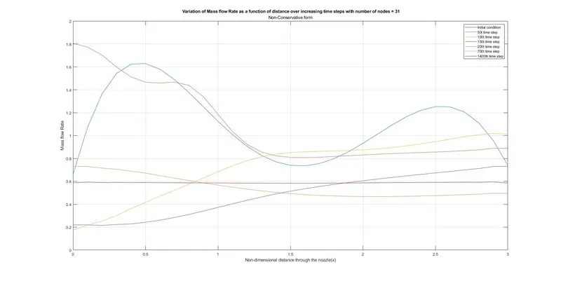
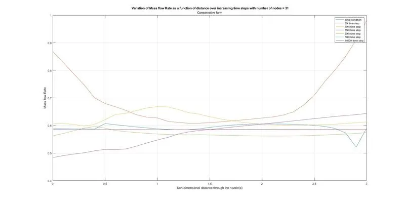
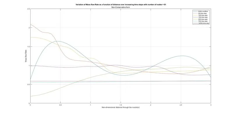
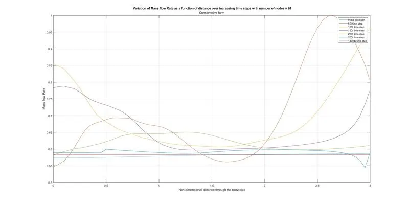
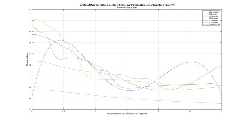
1) Variation of Mass flow Rate as a function of distance over increasing time steps with a varying number of nodes:
Non-Conservative and Conservative form:
Number of nodes(n)=31
NC:
C:
Number of nodes(n)=61
NC:
C:
Number of nodes(n)=91
NC:
C:
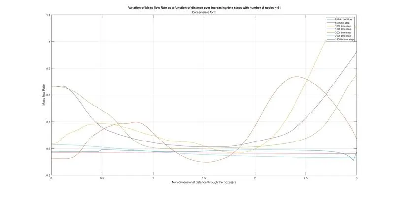
Inference: It is observed that the mass flow rate converges to a single line for the 1400th time step for both the conservative and non-conservative forms. It is also noted that the fluctuations are greater in the non-conservative form, while the conservative form is more stable and varies only slightly within a minimal range of primitive variable values.
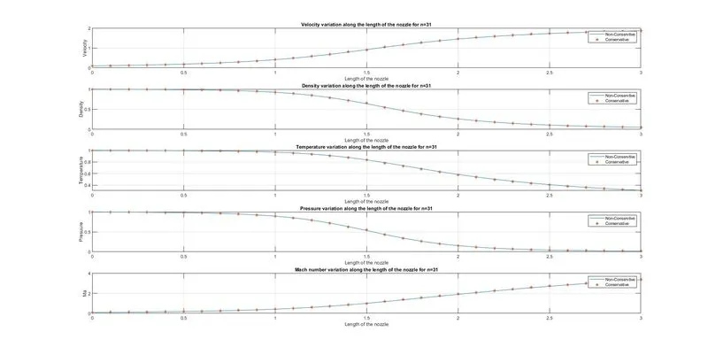
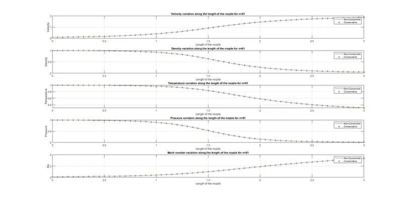
2) Variation of Primitive variables along the length of the nozzle for a varying number of nodes:
Number of nodes(n)=31
Number of nodes(n)=61
Number of nodes(n)=91
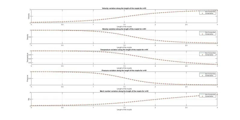
Inference: It is observed that, even though the number of nodes varies, the conservative and non-conservative forms yield the same results of the primitive variables at all the nodal points along the length of the nozzle after the 1400th time step.
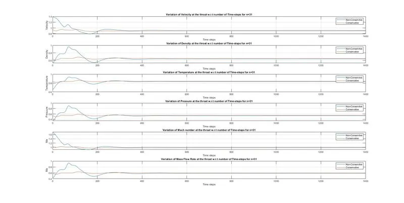
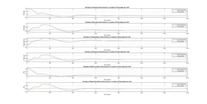
3) Variation of primitive variables at throat section as a function of increasing time steps with a varying number of nodes:
Number of nodes(n)=31
Number of nodes(n)=61
Number of nodes(n)=91
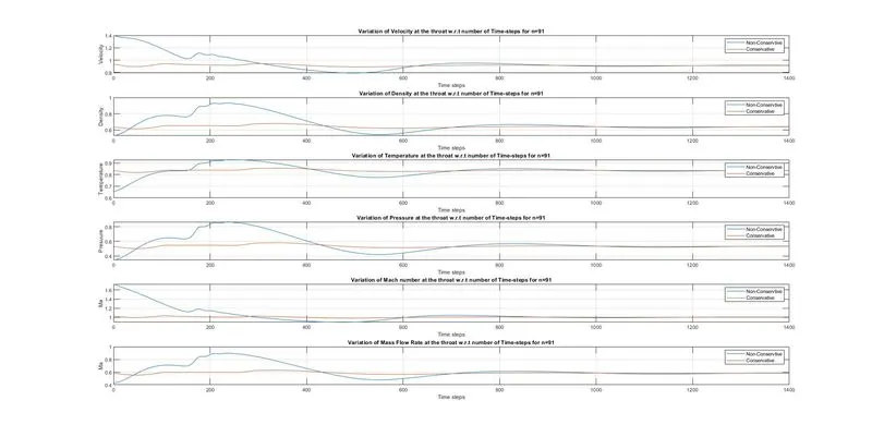
Inference: It is observed that the initial fluctuations become higher in the increasing order of the number of nodes, while eventually dies out and converges after 600, 800, and 1000 timesteps for n=31, 61, and 91 respectively. The aforesaid fluctuations did only occur in the non-conservative form, while the conservative form still remains stable till the end time step.
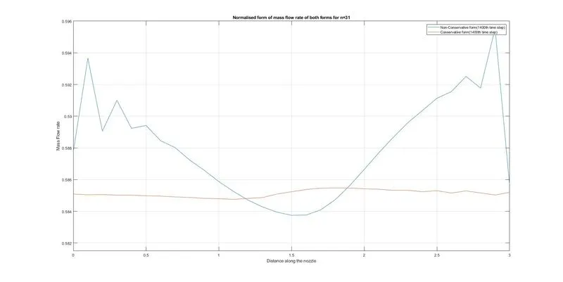
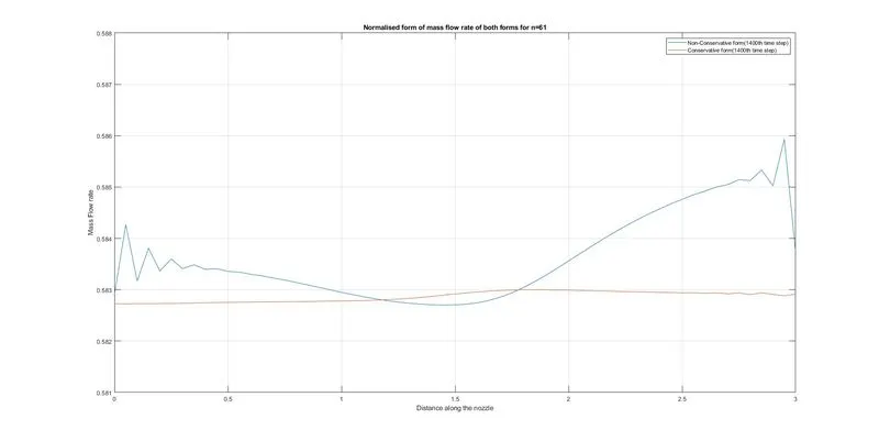
4) Comparison of Normalized mass flow rate distributions of both forms:
Number of nodes(n)=31
Number of nodes(n)=61
Number of nodes(n)=91
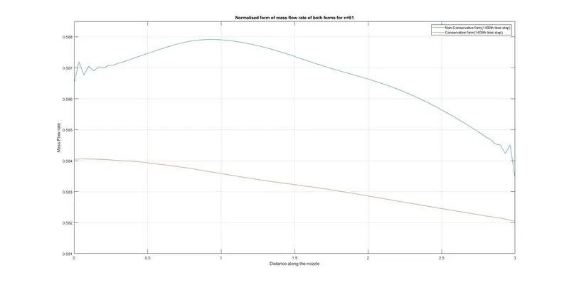
Inference: We hereby note that the conservative form yields a better stable result than that compared to the non-conservative form along the length of the nozzle. Even though it looks like we get the same value from the overall perspective, but when looking at it closer we see that the conservative form yields an accurate, and stable result.
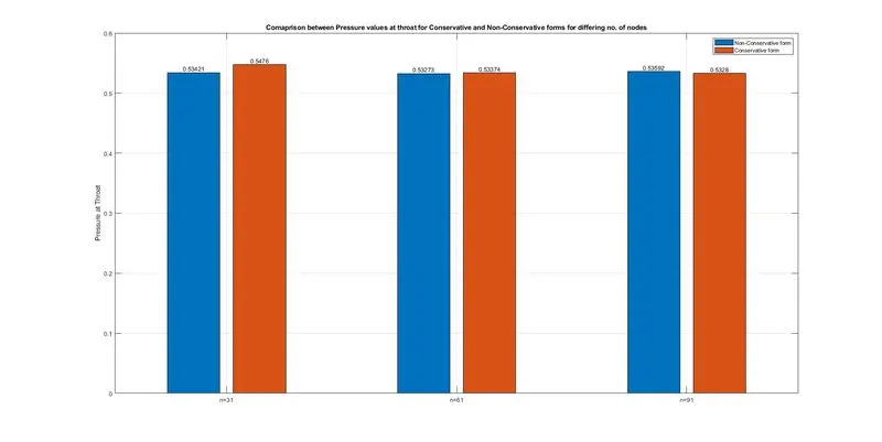
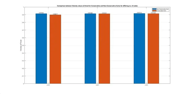
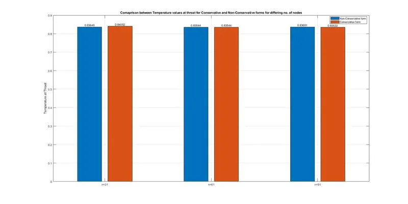
5) Grid independence test using bar plots for all the primitive variables:
Grid independence test for Pressure at the throat section:
Grid independence test for Velocity at the throat section:
Grid independence test for Temperature at the throat section:
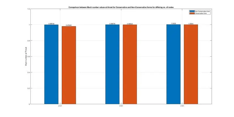
Grid independence test for Mach number at the throat section:
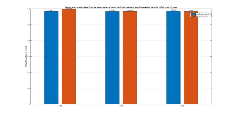
Grid independence test for Mass flow rate at the throat section:
Grid independence test for Density at the throat section:
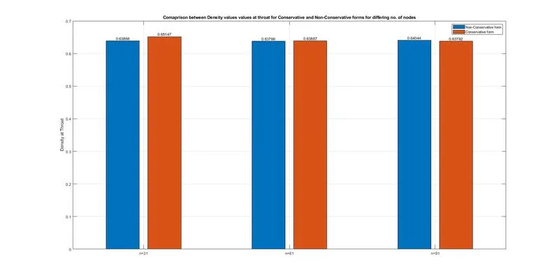
Inference: Grid dependency is an important factor, which at times affects the solution with a major impact on its convergence rate, stability, and accuracy. Thus when we look at the above results for all the primitive variables with their respective number of nodes as 31, 61, and 91, it is noted that there is not much difference between the final throat values which we get at the 1400th time step for the aforesaid differing number of nodes.
CONCLUSION:
Thus the simulation of the quasi-one-dimensional flow along the subsonic-supersonic nozzle using the MacCormack method for both Conservative and Non-Conservative forms concludes with the result that the conservative form yields the solution result with better stability and accuracy and also the results are validated to be of exactly correct values.