Week 12 - Validation studies of Symmetry BC vs Wedge BC in OpenFOAM vs Analytical H.P equation
From the previous challenge, we would have seen the usage of the wedge type Boundary Condition(BC), which is mainly used over the axisymmetric flow representing geometry like cylinders, which in general can be signified as, pipes, tubes, ducts, and other conduits. In this portion of the challenge, we would mainly look upon the usage of the Symmetry Boundary Condition(BC) in place of the Wedge BC and also do a comparative study analysis between both to identify the difference in results.
The main difference in between both the cases are tabulated below,
|
SI. No |
Wedge BC |
Symmetry BC |
|
1. |
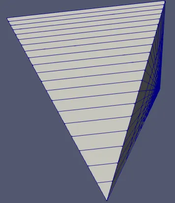
The wedge BC considers only a single straight mid-plane for a given wedge-shaped geometry(the triangular kind of looking shape) and represents the simulated values of the flow field variables only through that plane. (Note: The plane looks like when it is rotated 360 degrees it forms a full cylinder) |
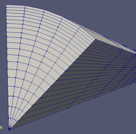
The symmetry BC is very similar to wedge BC in terms of visual perception but during the time of numerical analysis, it calculates the flow field variables for the complete cell volume rather than taking a single plane as in Wedge BC. |
|
2. |
Usage of Wedge BC limits our input value of a number of meshes along the wedge to be 1. Usage of many meshes in Wedge BC leads to errors in the result. The figure given below represents the 45deg wedge, using wedge BC.
|
The symmetry BC allows us to use multiple meshes keeping in mind the Courant number(more the meshes, lesser is the dx value), to be within the stability conditions. The figure given below represents the 45deg wedge, using Symmetry BC.
|
|
3. |
For the Wedge BC, as the angle changes for the same flow problem, the results also vary in its path of attaining the convergence. |
For the Symmetry BC, the angular changes that are considered don't affect or create an unsteady pattern for the path of attaining the convergence. |
The blockMeshdict file can be written for the wedge-angles of 100, 250, and 450 with the help of Matlab programming using the file parsing method as we have done in the previous challenge with the same input parameters which are given below,
- Reynolds Number = 2100 (Given)
- Diameter = 2cm = 0.02m (Assumed)
- Radius = 1cm = 0.01m
- Length_Entry(Le) = 0.05*Re*dia = 2.1m
- L = 3.1-2.1 = 1m
- Total length of the pipe = 2.1+1=3.1m
- Kinamatic Viscosity = 0.892e-6 m2/s(of water at 25deg celcius)
- Density of water(at 25 deg celsius) = 1000 Kg/m3
- Dynamic Viscosity = Kinematic Visc * density = 8.92e-04 Ns/(m2)
- Average Velocity = Kinematic Visc * Re / D = 0.0937 m/s
- Maximum velocity = 2*Average Velocity = 0.1873 m/s
- Angle of the wedge = 40
- Pressure loss =
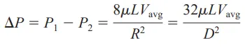 = 6.6836 Bar (Dynamic)
 - Kinematic Pressure loss= Dynamic Pressure loss / density = 0.0067 m^2/s^2
WRITING THE BLOCKMESHDICT FILE USING MATLAB:
The blockMeshdict file for 450 Symmetry BC is been given below as a Matlab code following the file parsing method.
clear all
close all
clc

Re=2100;    %given                                                         %reynolds number

d=0.02;     %meters                                                        %Dia of pipe
r=d/2;                                                                     %radius

len=0.05*Re*d;                                                             %length%until fully developed length
tot_len=len+1;                                                             %total length
nu=0.892e-6;                                                               %kinematic viscosity
rho=1000;                                                                  %density of water at 20deg celsius
mu=nu*rho;                                                                 %dynamic viscosity
v_avg=nu*Re/d;                                                             %Average velocity
v_max=2*v_avg;                                                             %Maximum velocity(Fully developed)
theta=input('Enter the theta(angle value) = ');                                                                   %Angle of the wedge:
del_p=(32*mu*(tot_len-len)*v_avg)/d^2;                                           %pressure loss
kin_p=del_p/rho;                                                           %kinetic pressure loss

%%
%vertices:
point0=[0 0 0];
point1=[0 r*cosd(theta/2) r*sind(theta/2)];
point2=[0 r*cosd(theta/2) -(r*sind(theta/2))];
point3=[tot_len 0 0];
point4=[tot_len r*cosd(theta/2) r*sind(theta/2)];
point5=[tot_len r*cosd(theta/2) -(r*sind(theta/2))];
%%
f2=fopen('blockMeshDict_symmetry_45.txt','w');                                         %Creating a blockMesh dict file in Notepad
fprintf(f2,'%sn','/*--------------------------------*- C++ -*----------------------------------*');
fprintf(f2,'%sn','=========                 |');
fprintf(f2,'%sn','  \      /  F ield         | OpenFOAM: The Open Source CFD Toolbox');
fprintf(f2,'%sn','   \    /   O peration     | Website:  https://openfoam.org');
fprintf(f2,'%sn','    \  /    A nd           | Version:  8');
fprintf(f2,'%sn','     \/     M anipulation  |');
fprintf(f2,'%sn','*---------------------------------------------------------------------------*/');
fprintf(f2,'%sn','FoamFile');
fprintf(f2,'%sn','{');
fprintf(f2,'%sn','    version     2.0;');
fprintf(f2,'%sn','    format      ascii;');
fprintf(f2,'%sn','    class       dictionary;');
fprintf(f2,'%sn','    object      blockMeshDict;');
fprintf(f2,'%sn','}');
fprintf(f2,'%sn','// * * * * * * * * * * * * * * * * * * * * * * * * * * * * * * * * * * * * * //');
fprintf(f2,'%sn',' ');
fprintf(f2,'%sn','convertToMeters 1;');
fprintf(f2,'%sn',' ');
fprintf(f2,'%sn','vertices');
fprintf(f2,'%sn','(');
fprintf(f2,'%s%f %f %f%sn','(',point0(1), point0(2), point0(3),')');
fprintf(f2,'%s%f %f %f%sn','(',point1(1), point1(2), point1(3),')');
fprintf(f2,'%s%f %f %f%sn','(',point2(1), point2(2), point2(3),')');
fprintf(f2,'%s%f %f %f%sn','(',point3(1), point3(2), point3(3),')');
fprintf(f2,'%s%f %f %f%sn','(',point4(1), point4(2), point4(3),')');
fprintf(f2,'%s%f %f %f%sn','(',point5(1), point5(2), point5(3),')');
fprintf(f2,'%sn',');');
fprintf(f2,'%sn',' ');
fprintf(f2,'%sn','blocks');
fprintf(f2,'%sn','(');
fprintf(f2,'%sn','    hex (0 3 5 2 0 3 4 1) (200 20 5) simpleGrading (1 0.2 1)');
fprintf(f2,'%sn',');');
fprintf(f2,'%sn',' ');
fprintf(f2,'%sn','edges');
fprintf(f2,'%sn','(');
fprintf(f2,'%s %s %s %s%f %f %f%sn','    arc', '1', '2', '(',0, r, 0,')');
fprintf(f2,'%s %s %s %s%f %f %f%sn','    arc', '4', '5', '(',tot_len, r, 0,')');
fprintf(f2,'%sn',');');
fprintf(f2,'%sn',' ');
fprintf(f2,'%sn','boundary');
fprintf(f2,'%sn','(');
fprintf(f2,'%sn','    inlet');
fprintf(f2,'%sn','    {');
fprintf(f2,'%sn','         type patch;');
fprintf(f2,'%sn','        faces');
fprintf(f2,'%sn','        (');
fprintf(f2,'%sn','             (0 1 2 0)');
fprintf(f2,'%sn','        );');
fprintf(f2,'%sn','    }');
fprintf(f2,'%sn','    outlet');
fprintf(f2,'%sn','     {');
fprintf(f2,'%sn','         type patch;');
fprintf(f2,'%sn','         faces');
fprintf(f2,'%sn','         (');
fprintf(f2,'%sn','            (3 5 4 3)');
fprintf(f2,'%sn','         );');
fprintf(f2,'%sn','    }');
fprintf(f2,'%sn','    Front');
fprintf(f2,'%sn','    {');
fprintf(f2,'%sn','        type symmetry;');
fprintf(f2,'%sn','        faces');
fprintf(f2,'%sn','         (');
fprintf(f2,'%sn','           (0 3 4 1)');
fprintf(f2,'%sn','        );');
fprintf(f2,'%sn','    }');
fprintf(f2,'%sn','    Back');
fprintf(f2,'%sn','    {');
fprintf(f2,'%sn','        type symmetry;');
fprintf(f2,'%sn','        faces');
fprintf(f2,'%sn','        (');
fprintf(f2,'%sn','	   (0 2 5 3)');
fprintf(f2,'%sn','        );');
fprintf(f2,'%sn','    }');
fprintf(f2,'%sn','    top');
fprintf(f2,'%sn','    {');
fprintf(f2,'%sn','    	type wall;');
fprintf(f2,'%sn','    	faces');
fprintf(f2,'%sn','    	(');
fprintf(f2,'%sn','   	     (1 4 5 2)');
fprintf(f2,'%sn','    	);');
fprintf(f2,'%sn','    }');
fprintf(f2,'%sn','    axis');
fprintf(f2,'%sn','    {');
fprintf(f2,'%sn','    	type empty;');
fprintf(f2,'%sn','    	faces');
fprintf(f2,'%sn','    	(');
fprintf(f2,'%sn','    	     (0 3 3 0)');
fprintf(f2,'%sn','    	);');
fprintf(f2,'%sn','     }');
fprintf(f2,'%sn',');');
fprintf(f2,'%sn',' ');
fprintf(f2,'%sn','mergePatchPairs');
fprintf(f2,'%sn','(');
fprintf(f2,'%sn',');');
fprintf(f2,'%sn',' ');
fprintf(f2,'%sn',' // ************************************************************************* //');

WRITTEN BLOCKMESHDICT FILE(for 45deg symmetry BC):
/*--------------------------------*- C++ -*----------------------------------*
=========                 |
  \      /  F ield         | OpenFOAM: The Open Source CFD Toolbox
   \    /   O peration     | Website:  https://openfoam.org
    \  /    A nd           | Version:  8
     \/     M anipulation  |
*---------------------------------------------------------------------------*/
FoamFile
{
    version     2.0;
    format      ascii;
    class       dictionary;
    object      blockMeshDict;
}
// * * * * * * * * * * * * * * * * * * * * * * * * * * * * * * * * * * * * * //

convertToMeters 1;

vertices
(
(0.000000 0.000000 0.000000)
(0.000000 0.009239 0.003827)
(0.000000 0.009239 -0.003827)
(3.100000 0.000000 0.000000)
(3.100000 0.009239 0.003827)
(3.100000 0.009239 -0.003827)
);

blocks
(
    hex (0 3 5 2 0 3 4 1) (200 20 5) simpleGrading (1 0.2 1)
);

edges
(
    arc 1 2 (0.000000 0.010000 0.000000)
    arc 4 5 (3.100000 0.010000 0.000000)
);

boundary
(
    inlet
    {
         type patch;
        faces
        (
             (0 1 2 0)
        );
    }
    outlet
     {
         type patch;
         faces
         (
            (3 5 4 3)
         );
    }
    Front
    {
        type symmetry;
        faces
         (
           (0 3 4 1)
        );
    }
    Back
    {
        type symmetry;
        faces
        (
	   (0 2 5 3)
        );
    }
    top
    {
    	type wall;
    	faces
    	(
   	     (1 4 5 2)
    	);
    }
    axis
    {
    	type empty;
    	faces
    	(
    	     (0 3 3 0)
    	);
     }
);

mergePatchPairs
(
);

 // ************************************************************************* //
CONTROLDICT FILE:
The Controldict file is been set up in such a way that it accepts the stability criteria of the CFL condition with giving suitable values for deltaT, and thus write the result at a regular interval of 20-time steps.
/*--------------------------------*- C++ -*----------------------------------*
  =========                 |
  \      /  F ield         | OpenFOAM: The Open Source CFD Toolbox
   \    /   O peration     | Website:  https://openfoam.org
    \  /    A nd           | Version:  8
     \/     M anipulation  |
*---------------------------------------------------------------------------*/
FoamFile
{
    version     2.0;
    format      ascii;
    class       dictionary;
    location    "system";
    object      controlDict;
}
// * * * * * * * * * * * * * * * * * * * * * * * * * * * * * * * * * * * * * //

application     icoFoam;

startFrom       startTime;

startTime       0;

stopAt          endTime;

endTime         50;

deltaT          0.01;

writeControl    timeStep;

writeInterval   20;

purgeWrite      0;

writeFormat     ascii;

writePrecision  6;

writeCompression off;

timeFormat      general;

timePrecision   6;

runTimeModifiable true;

adjustTimeStep    true;

maxCo	2;

maxDeltaT	0.1;


// ************************************************************************* //
PRESSURE FILE:
The Boundary Conditions for pressure are given such that the inlet BC is given zero gradient BC, thus assuming zero divergence factor at the inlet, and at the outlet, the BC of fixedValue was given with a value of 0.0067 m2 /s2, which is the value of Kinematic Pressure calculated in the previous sections from the Haigen-Poisuelle law's equation to find the Pressure loss.
/*--------------------------------*- C++ -*----------------------------------*
  =========                 |
  \      /  F ield         | OpenFOAM: The Open Source CFD Toolbox
   \    /   O peration     | Website:  https://openfoam.org
    \  /    A nd           | Version:  8
     \/     M anipulation  |
*---------------------------------------------------------------------------*/
FoamFile
{
    version     2.0;
    format      ascii;
    class       volScalarField;
    object      p;
}
// * * * * * * * * * * * * * * * * * * * * * * * * * * * * * * * * * * * * * //

dimensions      [0 2 -2 0 0 0 0];

internalField   uniform 0;

boundaryField
{
    inlet
    {
        type            zeroGradient;
    }
    outlet
    {
        type            fixedValue;
        value		 uniform 0.0067;
    }

    top
    {
        type            zeroGradient;
    }

    Front
    {
        type            wedge;
    }
    Back
    {
        type            wedge;
    }
    axis
    {
    	type		 empty;
    }
}
VELOCITY FILE:
The Boundary Conditions for velocity are given such that the inlet BC is given fixedValue BC, and was given with a value of 0.0937m/s which is the average velocity value obtained from the analytical equations above, and at the outlet, the BC of zeroGradient was used having zero divergence factor at the outlet.
/*--------------------------------*- C++ -*----------------------------------*
  =========                 |
  \      /  F ield         | OpenFOAM: The Open Source CFD Toolbox
   \    /   O peration     | Website:  https://openfoam.org
    \  /    A nd           | Version:  8
     \/     M anipulation  |
*---------------------------------------------------------------------------*/
FoamFile
{
    version     2.0;
    format      ascii;
    class       volVectorField;
    object      U;
}
// * * * * * * * * * * * * * * * * * * * * * * * * * * * * * * * * * * * * * //

dimensions      [0 1 -1 0 0 0 0];

internalField   uniform (0.0937 0 0);

boundaryField
{
    inlet
    {
        type            fixedValue;
        value           uniform (0.0937 0 0);
    }
    outlet
    {
        type            zeroGradient;
    }


    top
    {
        type            noSlip;
    }

    Front
    {
        type            wedge;
    }
    Back
    {
        type            wedge;
    }
    axis
    {
    	type		 empty;
    }
}

// ************************************************************************* //
Similarly, we set up the Symmetry BCs for the Wedge angle of 100, 250 and their mesh structures are given below in the image.
Angle=100, Symmetry BC:
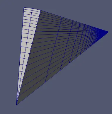 Here the number of cells is restricted to 2 in order to maintain the Courant number value less than 1.
Angle=250, Symmetry BC:
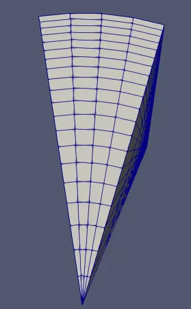 Here the number of cells is restricted to 4 in order to maintain the Courant number value less than 1.
RESULTS:
POST-PROCESSING VALIDATION OF VELOCITY:
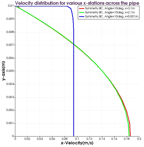
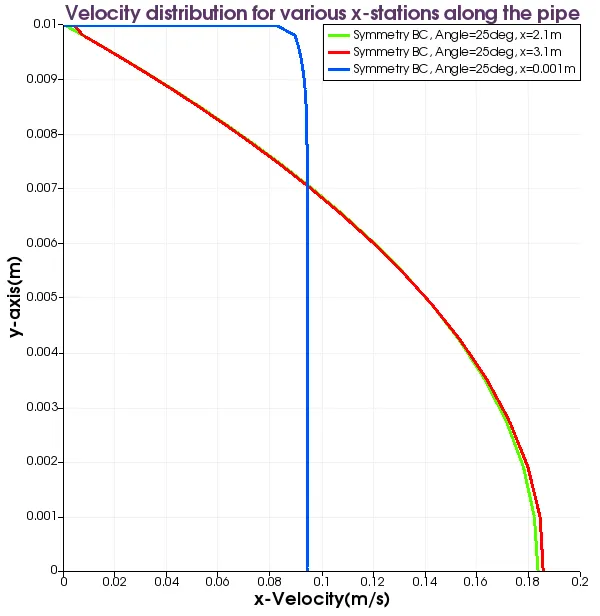
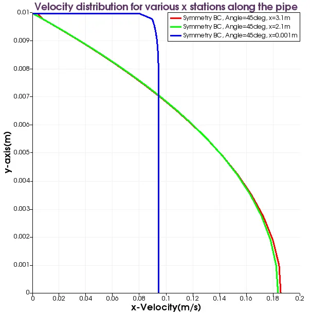
The Velocity profiles are obtained from each of the angles for both Wedge BC and Symmetry BC which are given individually below.
Individual Plots:
| Angle | Wedge | Symmetry |
| 100 | 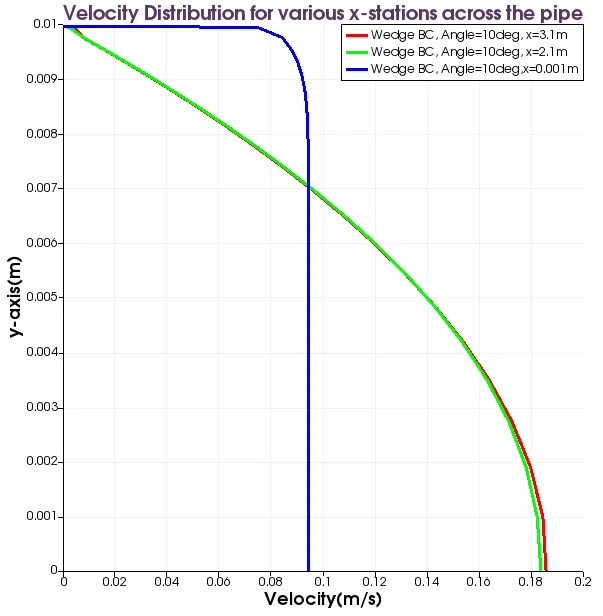 |
 |
| 250 | 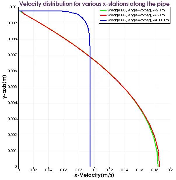 |
 |
| 450 | 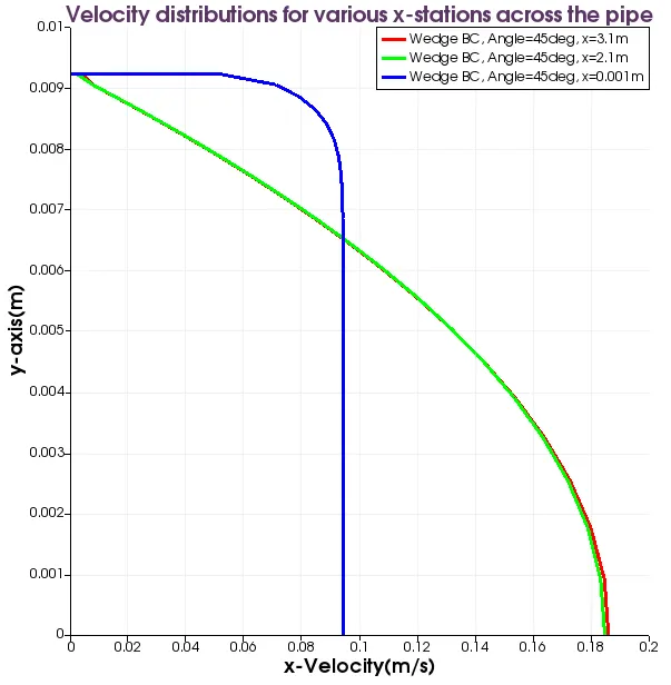 |
 |
Analytical plot:
Here we write a Matlab Code to come up with an analytical result at x=3.1m(Fully developed region) in order for us to validate the numerical solution result with it.
MatLab Code:
clear all
close all
clc
del_p=20.7191;
mu=8.92e-04;
R=0.01;
r=linspace(0,R,20);
l=3.1;
    for j=1:length(r)
        vel(j)=(del_p./(4*mu.*l))*(R^2)*(1-(r(j)^2 ./ R^2));
    end
figure(1)
plot(vel,r,'linewidth',2,'color','r')
title('Analytical Velocity Profile')
xlabel('x-Velocity')
ylabel('Y-axis(m)')
legend('x=3.1m')
grid on 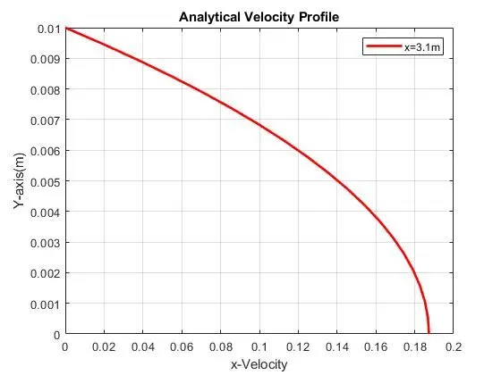
Comparison Plots:
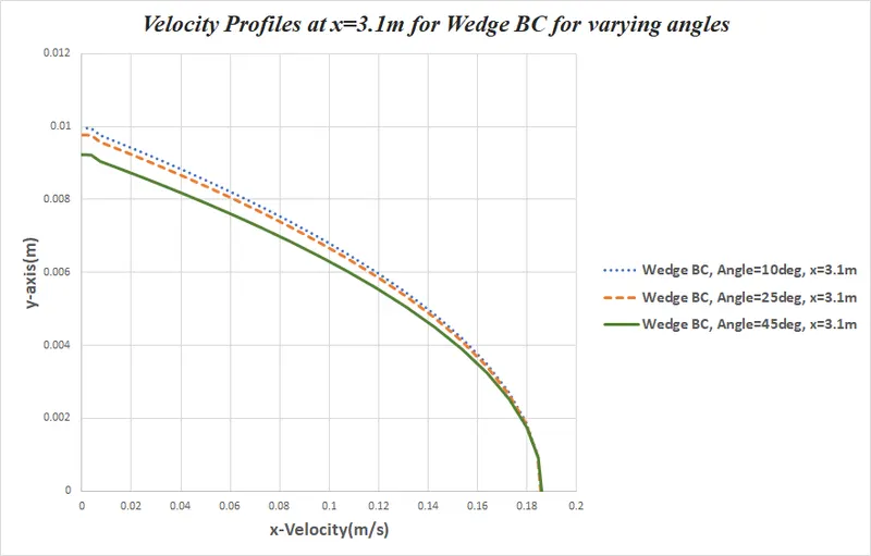
The data from the ParaView for the velocities at their corresponding arc lengths were taken at x=3.1m and were thus imported in Excel to make a comparative study.
| Wedge | Symmetry |
 |
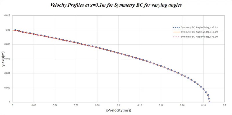 |
It is hereby inferred that, although any angular value choice is made, it is clear that the Symmetry BC yields an accurate result for all angles whereas, the Wedge BC yields an accurate result pathway only for the lower order of wedge angles.
The Analytical velocity value obtained from the formerly seen calculations is Maximum velocity(@x=3.1m)= 0.1873 m/s
The Velocity values obtained from the numerical analysis using OpenFoam are,
| Angle | Velocity(m/s) for Wedge | Velocity(m/s) for Symmetry |
| 100 | 0.185616 | 0.185602 |
| 250 | 0.185712 | 0.185604 |
| 450 | 0.185907 | 0.185612 |
From the above table too, it is inferred that the Symmetry BC has more or less an accurate result whereas, the Wedge BC has its result oscillating.
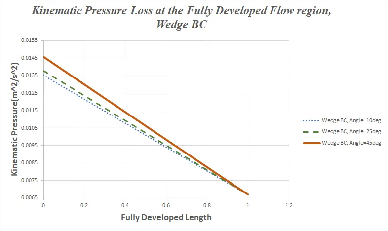
POST-PROCESSING AND VALIDATION OF KINEMATIC PRESSURE LOSS:
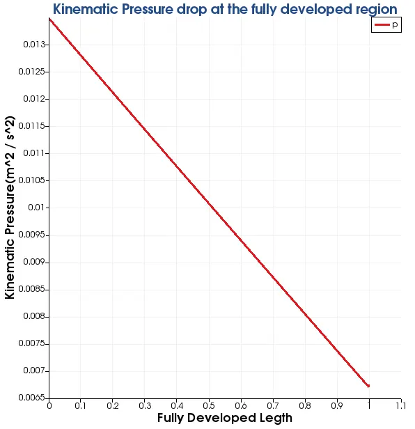
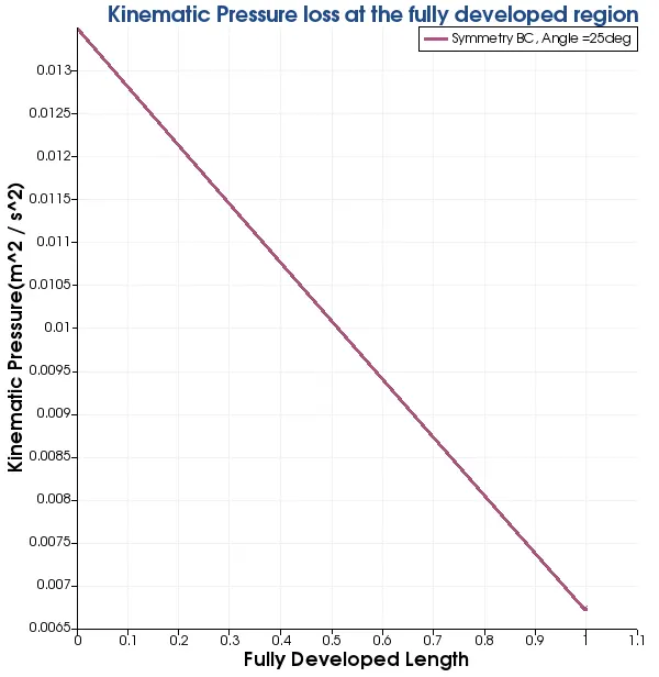
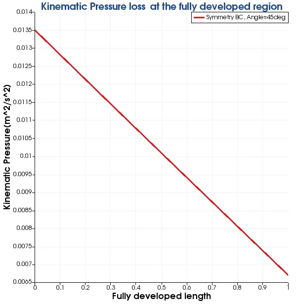
The Kinematic Pressure loss profiles are obtained from each of the angles for Wedge BC and Symmetry BC which are given individually below. The Kinematic Pressure loss is calculated for the fully developed region only, that is, x=2.1m is the starting of the fully developed region and the full length of the pipe is x=3.1m, so the region of interest to calculate the Kinematic Pressure loss is between 2.1m to 3.1m in the x-direction.
Individual Plots:
| Angle | Wedge | Symmetry |
| 100 | 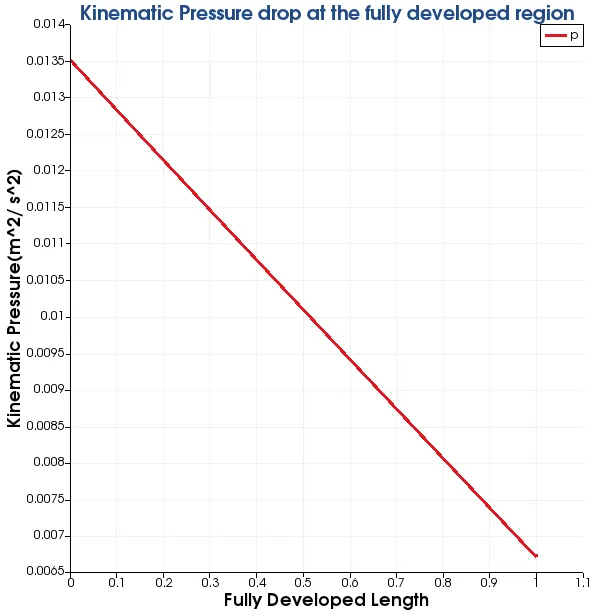 |
 |
| 250 | 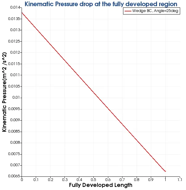 |
 |
| 450 | 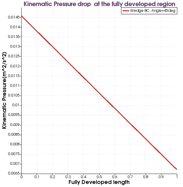 |
 |
Comparison Plots:
The data from the ParaView for the Kinematic Pressures between the region of interest were taken and were thus imported in Excel to make a comparative study.
| Wedge | Symmetry |
 |
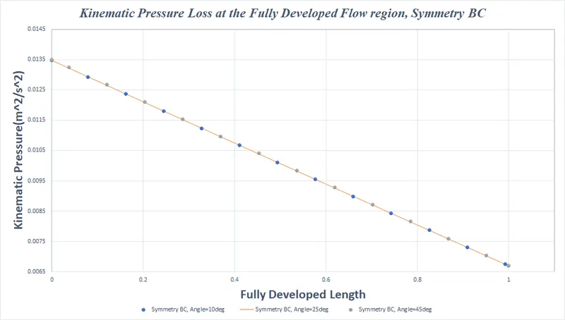 |
From the above comparison plots, we can witness that the Symmetry BC yields an accurate result for all the angles of the wedge, whereas the Wedge BC yields an accurate value pathway only for a lower-order angle.
The Analytical Value of Kinematic Pressure loss calculated from the formerly equations is Kinematic Pressure loss(between x=2.1m to 3.1m)= 0.0067 m^2/s^2
The Kinematic Pressure drop values obtained from the numerical analysis using OpenFoam are,
| Angle | Kinematic pressure drop(m^2 /s^2) for Wedge | Kinematic pressure drop(m^2 /s^2) for Symmetry |
| 100 | 0.00679 | 0.00672 |
| 250 | 0.00682 | 0.00680 |
| 450 | 0.00787 | 0.00676 |
Here too it is observed that there isn't any large variation of Kinematic Pressure drop for Symmetry BC, whereas for Wedge BC it shows an oscillating value, and this time the value for pressure for the highest angle is not that accurate when compared to what we inferred in velocity part. Hence using Wedge BC is at times uncertain.
POST-PROCESSING AND VALIDATION OF SHEAR STRESS PROFILES:
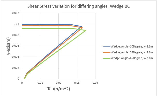
The Shear stress profiles for fully developed flow at x=2.1m are obtained for both Wedge and Symmetry BCs for the three different angles and are compared below.
Comparison Plots:
The data from the ParaView for the Shear stress @ x=2.1m(Fully developed flow stage) were taken and were thus imported in Excel to make a comparative study.
| Wedge | Symmetry |
 |
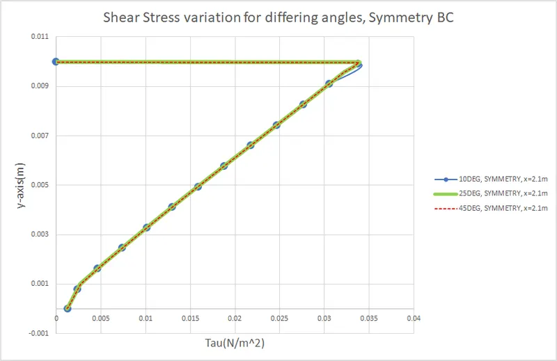 |
From the above plots, it is noted that the Shear stress plots for the Symmetry BC look accurate for all the angles, whereas the Wedge BC gives a variation of shear stress for differing angles.
Analytical plot:
The following image given below is a sample Analytical profile obtained from the velocity profile values calculated at x=2.1m and imported in MATLAB, then coded and given as a slightly unstable result.
MATLAB CODE:
clear all
close all
clc
mu=0.00089;
for i =1:(length(arc_length)-1)
    tau(i)= mu*((u(i+1)-u(i))/(arc_length(i+1)-arc_length(i)));
end
tau(1001)=0;
tau=tau';
plot(-tau,arc_length)
Where in the above CODE, arc_length, and u(velocity) are taken from the velocity profile values for Symmetry BC for Angle=45deg @ x=2.1m
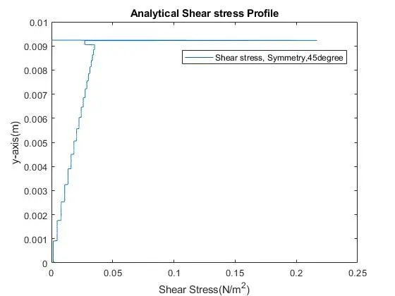
Neglecting the unstable plot the maximum shear stress can be concluded as 0.0335n/m^2.
Since it has some irregularities in its result the different BCs are compared with the numerical solution by means of values.
Comparison of Analytical Shear stress with the obtained Numerical Result:
| Angle | Shear stress(N/m^2) for Wedge BC | Shear stress(N/m^2) for Symmetry BC |
| 100 | 0.032376 | 0.0336816 |
| 250 | 0.0327737 | 0.03368 |
| 450 | 0.03574 | 0.0336745 |
From the above comparison, we can also conclude that the Symmetry BC yields an accurate result for Shear stress at all three angles, whereas the Wedge BC doesn't.