Week 3.5 - Deriving 4th order approximation of a 2nd order derivative using Taylor Table method

As from the previous challenges, we came to know that, the central differencing approach in numerical discretization has better accuracy towards the analytical value of the derivative when compared to the forward and backward differencing approaches. Similarly, we also saw that, as the order of approximation increases, the accuracy also rises.

Thus in this session, we would be involving both the above-mentioned cases for a 4th-order approximation of the second-order derivative of the function, f(x) = exp(x)*cos(x), wherein the errors must be comparatively studied for 3 types of numerical discretization methods, and they are,

1) Central Differencing method

2) Right-side skewed Differencing method

3) Left-side skewed Differencing method

Consider a stencil with n number of nodes or grid points. Now consider specific node i, and now when the node i is subjected to discretization, the central differencing method/approach gains information from its neighboring nodes from both sides, that is from (i-n)......i......(i+n). The Right-side skewed Differencing method gains information from only the nodes present on the right side of the node i, that is from i..........(i+n). This method is implemented for the node which is on the extreme left side beyond which no more grid points are found and nearer to the boundary. The Left-side skewed Differencing method gains information from only the nodes present on the left side of the node i, that is from (i-n)..........i. This method is implemented for the node which is on the extreme right side beyond which no more grid points are found and nearer to the boundary.

Here, the number of grid points considered in a stencil is different for different discretization methods i.e., the empirical relation between the N(number of grid points) and the methods of discretization are given below,

i) Central_differencing: Number of nodes in the stencil(N) = Order of Approximation(4th order) + Order of Derivative(2nd order) - 1

ii) Right and Left side skewed: Number of nodes in the stencil(N) = Order of Approximation(4th order) + Order of Derivative(2nd order)

Let us see the numerical derivative solution for the central, Skewed right-sided difference and Skewed left-sided difference by fixing the arbitrary constants for the functions at each point of the grid for a 4th-order Approximation of the second-order derivative of the function.

1) Central Differencing method:

For the central difference method, the procedure starts with the calculation of No. of nodes,

Number of nodes in the stencil(N) = Order of Approximation(4th order) + Order of Derivative(2nd order) - 1

Number of nodes in the stencil(N) = 4 + 2 - 1= 5

Therefore, the number of nodes is 5 and they are designated as, f(i-2)...f(i)...f(i+2)

∂2f/∂x2 = (af(i) + bf(i+1) + cf(i+2) + df(i+3) + ef(i+4) + gf(i+5) )/(dx^2)

The individual terms will be expanded with their coefficients being multiplied to the terms inside the taylor series expansion of each term.

The 5 equations comprising the 5 unknown coefficients(a,b,c,d,e,g) can be found from the following Taylor table.

	f(i)	f'(i).dx	f''(i).dx^2	f'''(i).dx^3	f''''(i).dx^4	f'''''(i).dx^5
af(i-2)	a	a(-2)	2a	a(-8/6)	a(16/24)	a(-32/120)
bf(i-1)	b	b(-1)	b/2	b(-1/6)	b(1/24)	b(-1/120)
cf(i)	c	0	0	0	0	0
df(i-1)	d	d	d/2	d(1/6)	d(1/24)	d(1/120)
ef(i+2)	e	2e	2e	e(8/6)	e(16/24)	e(32/120)
	0	0	1	0	0	?

The first 5 equations are formed by equating the first 5 columns to 0,0,1,0,0. The equations are formed by the basis of matrix form and the unknowns are identified by the matrix inversion method.

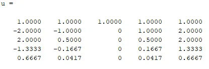
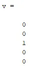
Assume, z as a (5x1)matrix of unknown coefficients, w= inv(u) * v

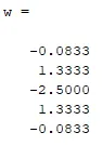
Therefore, the coefficients a=-0.0833, b=1.3333, c=-2.5, d=1.3333, and e=-0.0833

Hence the Central Differencing numerical method for the 4th-order approximation for the second-order derivative of the given function is represented by,

∂2f/∂x2 = ((-0.0833)f(i-2) + (1.3333)f(i-1) + (-2.5)f(i) + (1.3333)f(i+1) + (-0.0833)f(i+2)

2) Right-side skewed Differencing method:

For the right side skewed difference method, the procedure starts with the calculation of No. of nodes,

Number of nodes in the stencil(N) = Order of Approximation(4th order) + Order of Derivative(2nd order)

Number of nodes in the stencil(N) = 4 + 2 = 6

Therefore, the number of nodes is 6 and they are designated as, f(i)......f(i+5)

∂2f/∂x2 = (af(i) + bf(i+1) + cf(i+2) + df(i+3) + ef(i+4) + gf(i+5) )/(dx^2)

The individual terms will be expanded with their coefficients being multiplied to the terms inside the taylor series expansion of each term.

The 6 equations comprising the 6 unknown coefficients(a,b,c,d,e,g) can be found from the following Taylor table.

	f(i)	f'(i).dx	f''(i).dx^2	f'''(i).dx^3	f''''(i).dx^4	f'''''(i).dx^5	f''''''(i).dx^6
af(i)	a	0	0	0	0	0	0
bf(i+1)	b	b	b/2!	b/3!	b/4!	b/5!	b/6!
cf(i+2)	c	2c	4c/2!	8c/3!	16c/4!	32c/5!	64c/6!
df(i+3)	d	3d	9d/2!	27d/3!	81d/4!	243d/5!	729d/6!
ef(i+4)	e	4e	16e/2!	64e/3!	256e/4!	1024e/5!	4096e/6!
gf(i+5)	g	5g	25g/2!	125g/3!	625g/4!	3125g/5!	15625g/6!
	0	0	1	0	0	0	?

The first 6 equations are formed by equating the first 6 columns to 0,0,1,0,0,0. The equations are formed by the basis of matrix form and the unknowns are identified by the matrix inversion method.

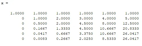
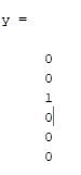
Assume, z as a (6x1)matrix of unknown coefficients, z= inv(x) * y

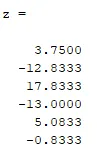
Therefore, the coefficients a=3.7500, b=-12.8333, c=17.8333, d=-13, e=5.0833, and g=-0.8333.

Hence the Right-side skewed Differencing numerical method for the 4th-order approximation for the second-order derivative of the given function is represented by,

∂2f/∂x2 = ((3.75)f(i) + (-12.8333)f(i+1) + (17.8333)f(i+2) + (-13)f(i+3) + (5.0833)f(i+4) + (-0.8333)f(i+5))/(dx^2)

3)Left-side skewed Differencing method:

For the left side skewed difference method, the procedure starts with the calculation of No. of nodes,

Number of nodes in the stencil(N) = Order of Approximation(4th order) + Order of Derivative(2nd order)

Number of nodes in the stencil(N) = 4 + 2 = 6

Therefore, the number of nodes is 6 and they are designated as, f(i-5)......f(i)

∂2f/∂x2 = (af(i-5) + bf(i-4) + cf(i-3) + df(i-2) + ef(i-1) + gf(i) )/(dx^2)

The individual terms will be expanded with their coefficients being multiplied to the terms inside the taylor series expansion of each term.

The 6 equations comprising the 6 unknown coefficients(a,b,c,d,e,g) can be found from the following Taylor table.

	f(i)	f'(i).dx	f''(i).dx^2	f'''(i).dx^3	f''''(i).dx^4	f'''''(i).dx^5	f''''''(i).dx^6
af(i-5)	a	a(-5)	a(25/2)	a(-125/6)	a(625/24)	a(-3125/120)	a(15625/720)
bf(i-4)	b	b(-4)	8b	b(-64/6)	b(256/24)	b(-1024/120)	b(4096/720)
cf(i-3)	c	c(-3)	c(9/2)	c(-27/6)	c(81/24)	c(-243/120)	c(729/720)
df(i-2)	d	d(-2)	d(4/2)	d(-8/6)	d(16/24)	d(-32/120)	d(64/720)
ef(i-1)	e	e(-1)	e(1/2)	e(-1/6)	e(1/24)	e(-1/120)	e(1/720)
gf(i)	g	0	0	0	0	0	0
	0	0	1	0	0	0	?

The first 6 equations are formed by equating the first 6 columns to 0,0,1,0,0,0. The equations are formed by the basis of matrix form and the unknowns are identified by the matrix inversion method.

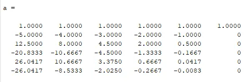
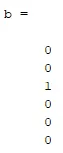
Assume, z as a (6x1)matrix of unknown coefficients, c= inv(a) * b

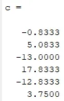
Therefore, the coefficients a=-0.8333, b=5.0833, c=-13, d=17.8333, e=-12.8333, and g=3.75.

Hence the Le-side skewed Differencing numerical method for the 4th-order approximation for the second-order derivative of the given function is represented by,

∂2f/∂x2 = ((-0.8333)f(i-5) + (5.0833)f(i-4) + (-13)f(i-3) + (17.8333)f(i-2) + (-12.8333)f(i-1) + (3.75)f(i))/(dx^2)

MATLAB CODE:

clear all
close all
clc
%function: f(x) = (e^x)*(cosx)
%Analytical/Exact derivative for the second-order derivative of f(x)is,
%f''(x)=-2*(e^x)*sinx
%Assigning the value of x, and a range for dx:
x=pi/3;
dx= linspace(pi/4000,pi/4,30)';
%defining the analytical derivative value
analytic_value= -2*(exp(x))*sin(x);
%Calling the functions for central,right and left side skewed 4th order approximation:
for i=1:length(dx)
error_rsd_skewed_4th_order(i) = right_side_skewed(x,dx(i));
error_lsd_skewed_4th_order(i) = left_side_skewed(x,dx(i));
error_central_aprox(i) = central_approx(x,dx(i));
end
loglog(dx,error_rsd_skewed_4th_order,'linewidth',3)
hold on
loglog(dx,error_lsd_skewed_4th_order,'linewidth',3)
hold on
loglog(dx,error_central_aprox,'linewidth',3)
ylabel('Error')
xlabel('Values of dx')
title('Comparison between Central,Right and Left Side Skewed 4th Order Approximations')
legend('RIGHT SIDE SKEWED','LEFT SIDE SKEWED','CENTRAL APPROXIMATION')

Now we must call the designated functions, which are given as follows,

CENTRAL_DIFFERENCING:

function error_central_approx_4th_order = central_approx(x,dx)
analytic_value= -2*(exp(x))*sin(x);
e=[1,1,1,1,1; -2,-1,0,1,2;2,1/2,0,1/2,2;-8/6,-1/6,0,1/6,8/6;16/24,1/24,0,1/24,16/24];
f=[0,0,1,0,0]';
g= inv(e)*f;
%include the original terms in the matrix as like left and right side skewed to reduce the round off error
central_approx_4th_order =( (g(3)*(exp(x)*cos(x))) + (g(2)*exp(x+dx)*cos(x+dx)) +(g(1)*exp(x+(2*dx))*cos(x+(2*dx))) + (g(5)* exp(x-(2*dx))*cos(x-(2*dx))) + (g(4)*exp(x-dx)*cos(x-dx)))/(dx^2);
error_central_approx_4th_order = abs(central_approx_4th_order-analytic_value);%error value for particular dx.
end

RIGHT-SIDE SKEWED DIFFERENCING:

function error_rsd_skewed_4th_order = right_side_skewed(x,dx)
analytic_value= -2*(exp(x))*sin(x);
w=[1,1,1,1,1,1 ; 0,1,2,3,4,5 ; 0,1/2,2,9/2,8,25/2 ; 0,1/6,4/3,9/2,32/3,125/6 ; 0,1/24,2/3,81/24,256/24,625/24 ; 0,1/120,32/120,243/120,1024/120,3125/120]
y=[0,0,1,0,0,0]'
z= inv(w) * y
rsd_skewed_4th_order =( (z(1)*(exp(x)*cos(x))) + (z(2)*exp(x+dx)*cos(x+dx)) +(z(3)*exp(x+(2*dx))*cos(x+(2*dx))) + (z(4)* exp(x+(3*dx))*cos(x+(3*dx))) + (z(5)*exp(x+(4*dx))*cos(x+(4*dx))) + (z(6)*exp(x+(5*dx))*cos(x+(5*dx))))/(dx^2);
error_rsd_skewed_4th_order = abs(rsd_skewed_4th_order-analytic_value);%error value for particular dx.
end

LEFT-SIDE SKEWED DIFFERENCING:

function error_lsd_skewed_4th_order = left_side_skewed(x,dx)
analytic_value= -2*(exp(x))*sin(x);
a=[1,1,1,1,1,1; -5,-4,-3,-2,-1,0 ; 25/2,8,9/2,2,1/2,0; -125/6,-64/6,-27/6,-8/6,-1/6,0; 625/24,256/24,81/24,16/24,1/24,0 ; -3125/120,-1024/120,-243/120,-32/120,-1/120,0];
b=[0,0,1,0,0,0]';
c= inv(a) *b;
lsd_skewed_4th_order =( (c(6)*(exp(x)*cos(x))) + ((c(5))*exp(x-dx)*cos(x-dx)) +(c(4)*exp(x-(2*dx))*cos(x-(2*dx))) + (c(3)* exp(x-(3*dx))*cos(x-(3*dx))) + (c(2)*exp(x-(4*dx))*cos(x-(4*dx))) + (c(1)*exp(x-(5*dx))*cos(x-(5*dx))))/(dx^2);
error_lsd_skewed_4th_order = abs(lsd_skewed_4th_order-analytic_value);%error value for particular dx.
end

RESULT:

The following is a log-log graph comparing the errors of Central, Right side, and Left side skewed differencing methods over a range of dx(grid spacing size).

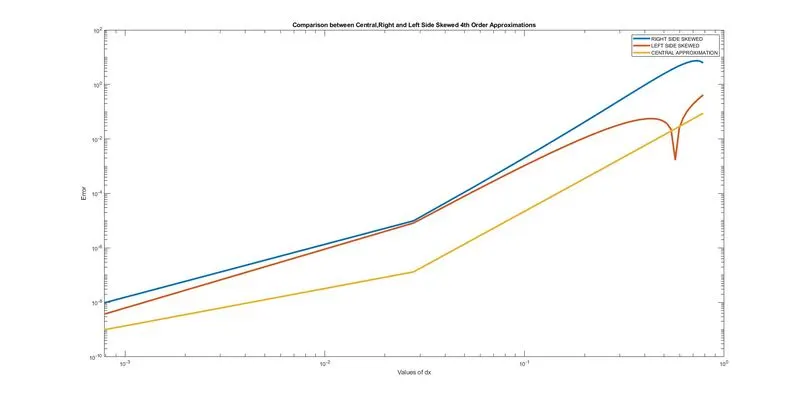
The error for the central differencing method is lesser than the other two.

INFERENCE:

As we can see from the above result, the following are the inferences made for the above problem statement,

1) The central difference method yields the most accurate result for the 4th-order approximation of the 2nd order derivative of any function when it is compared to the right or left-sided skewed differencing because central differencing takes information from both sides of the node while the right or left-sided skewed differencing takes information from only one side of them.

Why a skewed scheme is useful?

2) However, in situations like nearer to the boundary and left most grid point, then we must go for the right-sided skewed differencing method and vice versa for the left-sided skewed differencing method.

What can a skewed scheme do that a CD scheme cannot?

3) The work which the right and left-sided differencing methods do cannot be done by the central differencing method because central differencing cannot be applied at boundary nodes. Therefore both are equally important in terms of location of the grid point

NOTE: The derivations for the above calculations are attached with this report.