Week 11 - Simulation of Flow through a pipe in OpenFoam

SIMULATION OF FLOW THROUGH A PIPE IN OPENFOAM:

Internal Flow through a Pipe:

• Characteristics of the flow through a pipe

A flow through a pipe initially starts from a value of zero to the maximum velocity value at the center of the pipe, that is at the axis. The zero-velocity condition is mainly because of the no-slip condition prevailing near the walls or any stationary objectors. It is always convenient for us to use the average velocity values when it comes to the internal flow case scenarios, which generally remain as a constant for the same area in an incompressible type of flow. In the actual case, these flow field parameters including density, changes with temperature, but in practice, we consider them as constants for our convenience.

• Types of flows

Based on the type the flow is said to be, we split it into a dual case in practice, that is, 1) Laminar Flow, and 2)Turbulent Flow. The flow when following a smooth streamlined pathway with high orderliness motion is said to be Laminar Flow, while, when the flow is accompanied by high-velocity fluctuations and also high disorderliness, then it is said to be Turbulent Flow. In general, most flows that are encountered in real-life scenarios are of a Turbulent kind of nature, and Laminar flows are encountered in the flow of high viscous fluids. In between these two phases prevails a mid-phase, called as Transitional phase which exists only for a very little time, so which we do not consider it.

• Reynolds Number

The flow which is happening inside the pipe mainly depends on 2 types of forces, that is, 1)Inertial Forces, and 2)Viscous Forces. Thus the equation relating these two forces with the type of flow is given by the Reynolds number.

Reynolds Number = Inertial Force / Viscous Force

Re = Velocity_avg . Diameter / Kinematic Viscosity

= Density . Velocity_avg . Diameter / Dynamic Viscosity

At a higher Reynolds number, the inertial forces(which are proportional to the fluid density and square of the velocity), will be eventually higher causing fluctuations in the flow resulting in Turbulent Flow type and on the other hand when there is a lesser Reynolds number, the Viscous force dominates the inertial force thereby maintaining a smooth streamlined flow representing the laminar conditions.

Based on the above discussion, we conclude the values for Reynolds number for different types of flows as,

Re≤2300: Laminar Flow

2300≤Re≤4000: Transition Flow

Re≥4000: Turbulent Flow

• Entrance Region and Entry Length:

Considering the flow through the pipe, at the start of the flow, initially the fluid lines which are near o the walls experience a no-slip condition, wherein the flow does not happen and for this factor accompanied with the viscosity of the fluid, these fluid lines try to decrease the velocity of the adjacent fluid lines thus causing the formation of the Boundary layer. Thus in order to maintain the mass flow rate, it eventually happens to increase the velocity at the center of the pipe after a certain distance. This distance that is required for the fluid to reach its maximum velocity value at the center of the pipe is said to be Hydrodynamic Entrance Region, and the region covering the fully developed flow is called the Hydrodynamically Fully Developed flow.

For a Laminar flow, the Reynolds number for the Hydrodynamic Entry length of the pipe is given as {L(developing) / Diameter} = 0.05 . Re

The image given below picturizes the development of the boundary layer across the length of the pipe for a laminar flow condition defining the regions of developing and developed flows.

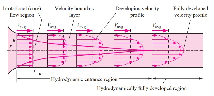
As discussed earlier, we assume the velocity value of the initial uniform cross-section of the velocity profile as Average Velocity. And thus, we keep relating the variation of the velocity profile with an equation given below.

u(r) = (Pressure loss / 4 . Dynamic Viscosity . Length of the pipe) . R². (1-(r/R)²)

And at last, we relate the maximum velocity with the average velocity as,

u(max) = 2 . Velocity_avg

• Shear stress Distribution

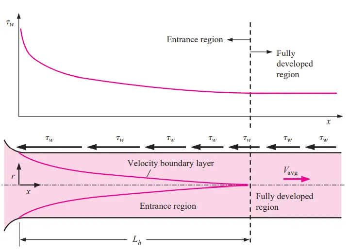
The shear stress is directly proportional to the Shear strain Rate of the Newtonian fluids and is generally related to the Viscosity of the fluid and the No-Slip condition existing around the walls of the flow section. Initially, at the entry region, the wall shear stress will be very large thus forming a non-variable velocity field along the Radial direction equal to Average velocity, and then eventually decreases and becomes a constant(reduced for all the points along the length after the formation of the fully developed hydrodynamic region).

• Pressure Drop for Laminar Flow:

Pressure loss is a general phenomenon happening inside a pipe, duct, tubes, etc., comprising a flow case scenario. Often the Pressure drop value gives the value of Power requirements to pump the sufficient pressurized water, for which the pressure is often indicated in terms of head, so that, the height of water to be raised(to be pumped) can be calculated.

In general, the Pressure loss relation for the flow is given by,

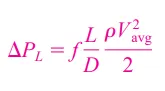where f is the Darcy friction factor, and the other term is called the dynamic pressure term.

The friction factor for circular pipe, and for Laminar flow, is given as, 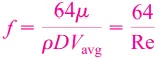where the type of flow is determined through Reynolds number.

And as said earlier, we indicate the pressure loss term often as Head loss, which is represented as,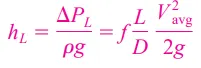

The relation between the pressure loss and Dynamic viscosity, Length of the pipe, Average Velocity, and Diameter is given by the Haigen-Poisuelle Equation, which is also known as Haigen-Poisuelle Law, which is applicable for incompressible, and Laminar flow of a Newtonian Fluid over a circular cross-section. The corresponding equation is given below.

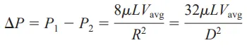
Values through Calculations and Assumptions:

• Reynolds Number = 2100 (Given)
• Diameter = 2cm = 0.02m (Assumed)
• Radius = 1cm = 0.01m
• Length(Entry) = 0.05*Re*dia = 2.1m
• Total length of the pipe = 2.1+1=3.1m
• Kinamatic Viscosity = 0.892e-6 m²/s(of water at 25deg celcius)
• Density of water(at 25 deg celsius) = 1000 Kg/m³
• Dynamic Viscosity = Kinematic Visc * density = 8.92e-04 Ns/(m²)
• Average Velocity = Kinematic Visc * Re / D = 0.0937 m/s
• Maximum velocity = 2*Average Velocity = 0.1873 m/s
• Angle of the wedge = 4⁰
• Pressure loss = = 20.7191 Bar (Dynamic)
• Kinematic Pressure loss= Dynamic Pressure loss / density = 0.0207 Bar

Creating the blockMeshDict file using Matlab:

The blockMeshDict file which is modifiable is created using MATLAB with the help of 'fopen' and 'w'~write command. The main reason why we prefer the writing of this blockMeshDict file using MATLAB is, we try to create a wedge-shaped geometry representing the pipe because the inclusion of the whole circular geometry causes enormous running time of the simulation, and it also requires more space. Thus we go for the wedge-shaped geometry method.

The wedge-shaped geometry is represented as in the picture below.

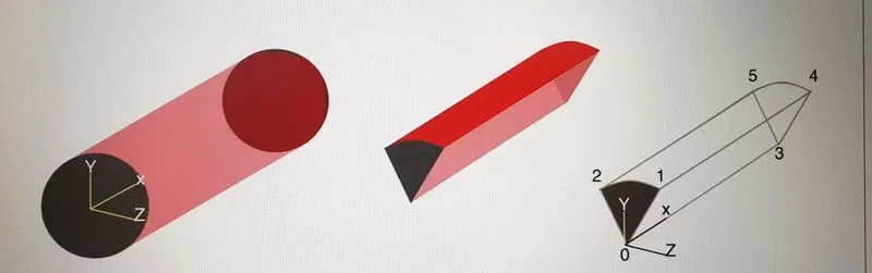
The vertices are the points representing the wedge geometry are represented inside the vertices column of the blockMeshDict file.

The y and z distance of the resolved radius from the azimuthal radius is represented as, rcos(θ/2) and rsin(θ/2), and the sign convention is included accordingly.

Thus the blockMeshDict file is written using the File parsing method through MATLAB to OpenFoam, which is represented below.

MAIN PROGRAM:

WRITING THE BLOCKMESH DICT FILE:

clear all
close all
clc

Re=2100;    %given                                                         %reynolds number

d=0.02;     %meters                                                        %Dia of pipe
r=d/2;                                                                     %radius

len=0.05*Re*d;                                                             %length%until fully developed length
tot_len=len+1;                                                             %total length
nu=0.892e-6;                                                               %kinematic viscosity
rho=1000;                                                                  %density of water at 25deg celsius
mu=nu*rho;                                                                 %dynamic viscosity
v_avg=nu*Re/d;                                                             %Average velocity
v_max=2*v_avg;                                                             %Maximum velocity(Fully developed)
theta=4;                                                                   %Angle of the wedge:
del_p=(32*mu*tot_len*v_avg)/d^2;                                           %pressure loss
kin_p=del_p/rho;                                                           %kinetic pressure loss

%%
%vertices:
point0=[0 0 0];
point1=[0 r*cosd(theta/2) r*sind(theta/2)];
point2=[0 r*cosd(theta/2) -(r*sind(theta/2))];
point3=[tot_len 0 0];
point4=[tot_len r*cosd(theta/2) r*sind(theta/2)];
point5=[tot_len r*cosd(theta/2) -(r*sind(theta/2))];
%%
f2=fopen('blockMeshDict.txt','w');                                         %Creating a blockMesh dict file in Notepad
fprintf(f2,'%s\n','/*--------------------------------*- C++ -*----------------------------------*\');
fprintf(f2,'%s\n','=========                 |');
fprintf(f2,'%s\n','  \\      /  F ield         | OpenFOAM: The Open Source CFD Toolbox');
fprintf(f2,'%s\n','   \\    /   O peration     | Website:  https://openfoam.org');
fprintf(f2,'%s\n','    \\  /    A nd           | Version:  8');
fprintf(f2,'%s\n','     \\/     M anipulation  |');
fprintf(f2,'%s\n','\*---------------------------------------------------------------------------*/');
fprintf(f2,'%s\n','FoamFile');
fprintf(f2,'%s\n','{');
fprintf(f2,'%s\n','    version     2.0;');
fprintf(f2,'%s\n','    format      ascii;');
fprintf(f2,'%s\n','    class       dictionary;');
fprintf(f2,'%s\n','    object      blockMeshDict;');
fprintf(f2,'%s\n','}');
fprintf(f2,'%s\n','// * * * * * * * * * * * * * * * * * * * * * * * * * * * * * * * * * * * * * //');
fprintf(f2,'%s\n',' ');
fprintf(f2,'%s\n','convertToMeters 1;');
fprintf(f2,'%s\n',' ');
fprintf(f2,'%s\n','vertices');
fprintf(f2,'%s\n','(');
fprintf(f2,'%s%f %f %f%s\n','(',point0(1), point0(2), point0(3),')');
fprintf(f2,'%s%f %f %f%s\n','(',point1(1), point1(2), point1(3),')');
fprintf(f2,'%s%f %f %f%s\n','(',point2(1), point2(2), point2(3),')');
fprintf(f2,'%s%f %f %f%s\n','(',point3(1), point3(2), point3(3),')');
fprintf(f2,'%s%f %f %f%s\n','(',point4(1), point4(2), point4(3),')');
fprintf(f2,'%s%f %f %f%s\n','(',point5(1), point5(2), point5(3),')');
fprintf(f2,'%s\n',');');
fprintf(f2,'%s\n',' ');
fprintf(f2,'%s\n','blocks');
fprintf(f2,'%s\n','(');
fprintf(f2,'%s\n','    hex (0 3 5 2 0 3 4 1) (200 20 1) simpleGrading (1 0.2 1)');
fprintf(f2,'%s\n',');');
fprintf(f2,'%s\n',' ');
fprintf(f2,'%s\n','edges');
fprintf(f2,'%s\n','(');
fprintf(f2,'%s %s %s %s%f %f %f%s\n','    arc', '1', '2', '(',0, r, 0,')');
fprintf(f2,'%s %s %s %s%f %f %f%s\n','    arc', '4', '5', '(',tot_len, r, 0,')');
fprintf(f2,'%s\n',');');
fprintf(f2,'%s\n',' '); 
fprintf(f2,'%s\n','boundary');
fprintf(f2,'%s\n','(');
fprintf(f2,'%s\n','    inlet');
fprintf(f2,'%s\n','    {');
fprintf(f2,'%s\n','         type patch;');
fprintf(f2,'%s\n','        faces');
fprintf(f2,'%s\n','        (');
fprintf(f2,'%s\n','             (0 1 2 0)');
fprintf(f2,'%s\n','        );');
fprintf(f2,'%s\n','    }');
fprintf(f2,'%s\n','    outlet');
fprintf(f2,'%s\n','     {');
fprintf(f2,'%s\n','         type patch;');
fprintf(f2,'%s\n','         faces');
fprintf(f2,'%s\n','         (');
fprintf(f2,'%s\n','            (3 5 4 3)');
fprintf(f2,'%s\n','         );');
fprintf(f2,'%s\n','    }');
fprintf(f2,'%s\n','    Front');
fprintf(f2,'%s\n','    {');
fprintf(f2,'%s\n','        type wedge;');
fprintf(f2,'%s\n','        faces');
fprintf(f2,'%s\n','         (');
fprintf(f2,'%s\n','           (0 3 4 1)');
fprintf(f2,'%s\n','        );');
fprintf(f2,'%s\n','    }');
fprintf(f2,'%s\n','    Back');
fprintf(f2,'%s\n','    {');
fprintf(f2,'%s\n','        type wedge;');
fprintf(f2,'%s\n','        faces');
fprintf(f2,'%s\n','        (');
fprintf(f2,'%s\n','	   (0 2 5 3)');
fprintf(f2,'%s\n','        );');
fprintf(f2,'%s\n','    }');
fprintf(f2,'%s\n','    top');
fprintf(f2,'%s\n','    {');
fprintf(f2,'%s\n','    	type wall;');
fprintf(f2,'%s\n','    	faces');
fprintf(f2,'%s\n','    	(');
fprintf(f2,'%s\n','   	     (1 4 5 2)');
fprintf(f2,'%s\n','    	);');
fprintf(f2,'%s\n','    }');
fprintf(f2,'%s\n','    axis');
fprintf(f2,'%s\n','    {');
fprintf(f2,'%s\n','    	type empty;');
fprintf(f2,'%s\n','    	faces');
fprintf(f2,'%s\n','    	(');
fprintf(f2,'%s\n','    	     (0 3 3 0)');
fprintf(f2,'%s\n','    	);');
fprintf(f2,'%s\n','     }');
fprintf(f2,'%s\n',');');
fprintf(f2,'%s\n',' '); 
fprintf(f2,'%s\n','mergePatchPairs');
fprintf(f2,'%s\n','(');
fprintf(f2,'%s\n',');');
fprintf(f2,'%s\n',' '); 
fprintf(f2,'%s\n',' // ************************************************************************* //');

WRITTEN BLOCKMESH DICT FILE:

The blockMesh Dict file must be written in the format that consists of the boundary types Inlet, Outlet, Front, and Back wedge, Wall, and Axis with their vertices being denoted with respect to the right-hand thumb rule. The edges must be represented as arcs specified as, arc 1 2, and arc 4 5. The mesh grading is done such that the walls comprise the dense number of cells corresponding to better capturing the results of the no-slip conditions.

/*--------------------------------*- C++ -*----------------------------------*\
=========                 |
  \\      /  F ield         | OpenFOAM: The Open Source CFD Toolbox
   \\    /   O peration     | Website:  https://openfoam.org
    \\  /    A nd           | Version:  8
     \\/     M anipulation  |
\*---------------------------------------------------------------------------*/
FoamFile
{
    version     2.0;
    format      ascii;
    class       dictionary;
    object      blockMeshDict;
}
// * * * * * * * * * * * * * * * * * * * * * * * * * * * * * * * * * * * * * //
 
convertToMeters 1;
 
vertices
(
(0.000000 0.000000 0.000000)
(0.000000 0.009994 0.000349)
(0.000000 0.009994 -0.000349)
(3.100000 0.000000 0.000000)
(3.100000 0.009994 0.000349)
(3.100000 0.009994 -0.000349)
);
 
blocks
(
    hex (0 3 5 2 0 3 4 1) (200 20 1) simpleGrading (1 0.2 1)
);
 
edges
(
    arc 1 2 (0.000000 0.010000 0.000000)
    arc 4 5 (3.100000 0.010000 0.000000)
);
 
boundary
(
    inlet
    {
         type patch;
        faces
        (
             (0 1 2 0)
        );
    }
    outlet
     {
         type patch;
         faces
         (
            (3 5 4 3)
         );
    }
    Front
    {
        type wedge;
        faces
         (
           (0 3 4 1)
        );
    }
    Back
    {
        type wedge;
        faces
        (
	   (0 2 5 3)
        );
    }
    top
    {
    	type wall;
    	faces
    	(
   	     (1 4 5 2)
    	);
    }
    axis
    {
    	type empty;
    	faces
    	(
    	     (0 3 3 0)
    	);
     }
);
 
mergePatchPairs
(
);
 
 // ************************************************************************* //

SETTING UP THE CONTROLDICT FILE:

The ControlDict file is set up such that the Courant number does not exceed the value of 1, by modifying the time-step value. We also indicate the results to be written exactly or 20 intervals each.

/*--------------------------------*- C++ -*----------------------------------*\
  =========                 |
  \\      /  F ield         | OpenFOAM: The Open Source CFD Toolbox
   \\    /   O peration     | Website:  https://openfoam.org
    \\  /    A nd           | Version:  8
     \\/     M anipulation  |
\*---------------------------------------------------------------------------*/
FoamFile
{
    version     2.0;
    format      ascii;
    class       dictionary;
    location    "system";
    object      controlDict;
}
// * * * * * * * * * * * * * * * * * * * * * * * * * * * * * * * * * * * * * //

application     icoFoam;

startFrom       startTime;

startTime       0;

stopAt          endTime;

endTime         50;

deltaT          0.01;

writeControl    timeStep;

writeInterval   20;

purgeWrite      0;

writeFormat     ascii;

writePrecision  6;

writeCompression off;

timeFormat      general;

timePrecision   6;

runTimeModifiable true;

adjustTimeStep    true;

maxCo	2;

maxDeltaT	0.1;


// ************************************************************************* //

SETTING UP INITIAL PRESSURE AND VELOCITY CONDITIONS:

PRESSURE:

Here we give zeroGradient for Inlet, thus satisfying the Neuman Boundary condition, and a fixed value of 0.0207Bar acquired from the Kinematic pressure loss from the analytical part is assumed as the outlet boundary field condition. And the other BCs are explainable on their own.

/*--------------------------------*- C++ -*----------------------------------*\
  =========                 |
  \\      /  F ield         | OpenFOAM: The Open Source CFD Toolbox
   \\    /   O peration     | Website:  https://openfoam.org
    \\  /    A nd           | Version:  8
     \\/     M anipulation  |
\*---------------------------------------------------------------------------*/
FoamFile
{
    version     2.0;
    format      ascii;
    class       volScalarField;
    object      p;
}
// * * * * * * * * * * * * * * * * * * * * * * * * * * * * * * * * * * * * * //

dimensions      [0 2 -2 0 0 0 0];

internalField   uniform 0;

boundaryField
{
    inlet
    {
        type            zeroGradient;
    }
    outlet
    {
        type            fixedValue;
        value		 uniform 0.0207;
    }

    top
    {
        type            zeroGradient;
    }

    Front
    {
        type            wedge;
    }
    Back
    {
        type            wedge;
    }
    axis
    {   
    	type		 empty;
    }
}

VELOCITY:

Here, the major change that we did is, we gave the fixed value of 0.0937m/s that we acquired from the analytical part of the calculation as the inlet fixed value BC.

/*--------------------------------*- C++ -*----------------------------------*\
  =========                 |
  \\      /  F ield         | OpenFOAM: The Open Source CFD Toolbox
   \\    /   O peration     | Website:  https://openfoam.org
    \\  /    A nd           | Version:  8
     \\/     M anipulation  |
\*---------------------------------------------------------------------------*/
FoamFile
{
    version     2.0;
    format      ascii;
    class       volVectorField;
    object      U;
}
// * * * * * * * * * * * * * * * * * * * * * * * * * * * * * * * * * * * * * //

dimensions      [0 1 -1 0 0 0 0];

internalField   uniform (0.0937 0 0);

boundaryField
{
    inlet
    {
        type            fixedValue;
        value           uniform (0.0937 0 0);
    }
    outlet
    {
        type            zeroGradient;
    }


    top
    {
        type            noSlip;
    }

    Front
    {
        type            wedge;
    }
    Back
    {
        type            wedge;
    }
    axis
    {
    	type		 empty;
    }
}

// ************************************************************************* //

SETTING UP THE TRANSPORT PROPERTIES:

The value of the Kinematic viscosity of the water at 25deg celsius is 0.892e-6, and the same is indicated inside this file.

/*--------------------------------*- C++ -*----------------------------------*\
  =========                 |
  \\      /  F ield         | OpenFOAM: The Open Source CFD Toolbox
   \\    /   O peration     | Website:  https://openfoam.org
    \\  /    A nd           | Version:  8
     \\/     M anipulation  |
\*---------------------------------------------------------------------------*/
FoamFile
{
    version     2.0;
    format      ascii;
    class       dictionary;
    location    "constant";
    object      transportProperties;
}
// * * * * * * * * * * * * * * * * * * * * * * * * * * * * * * * * * * * * * //

nu              [0 2 -1 0 0 0 0] 0.892e-6;


// ************************************************************************* //

MESHED GEOMETRY:

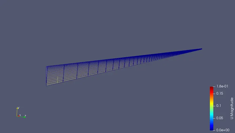
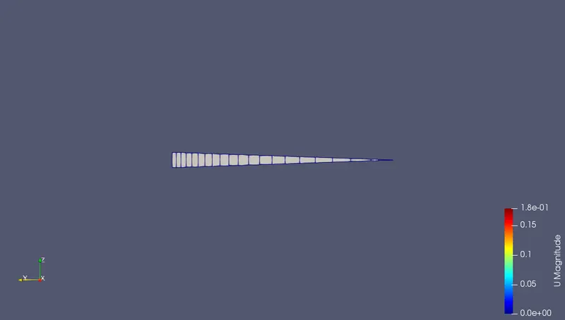
The mesh of the geometry is framed in such a way that the size of the volumes becomes thinner near the walls with more concentration of their numbers. Thus allowing better capture of the Boundary layer near the walls. The given mesh grading factor is (1 0.2 1).

The following figures below indicate the mesh structure of the wedge-shaped geometry.

VELOCITY DISTRIBUTION:

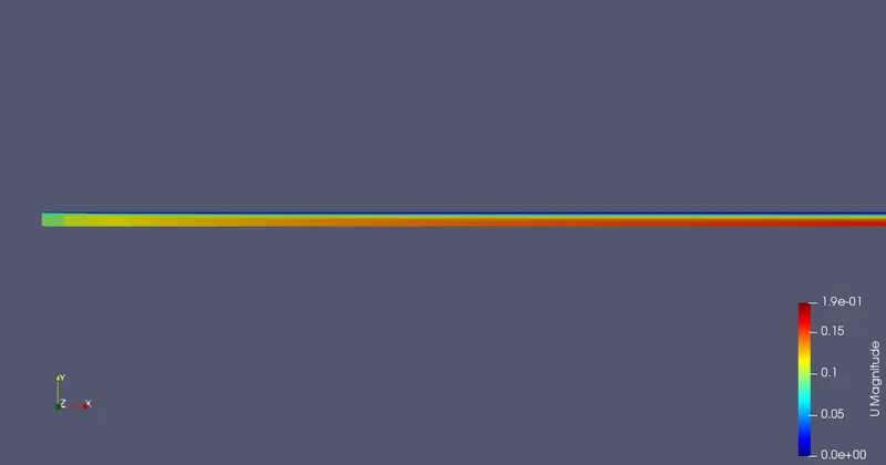
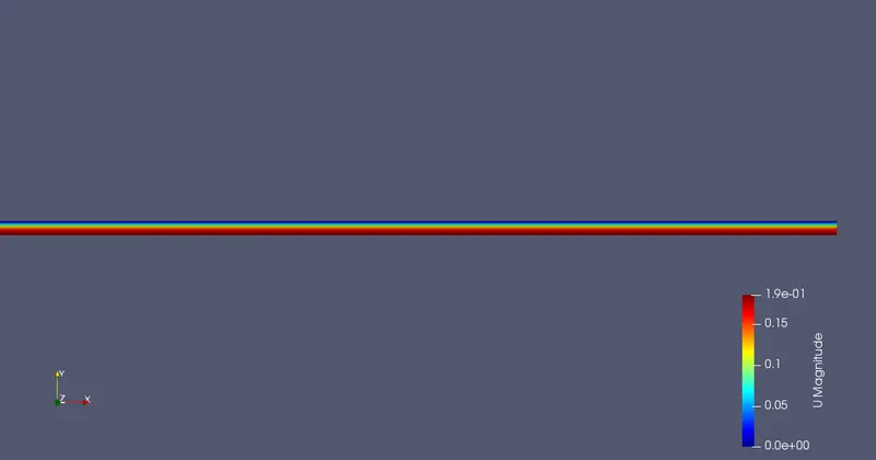
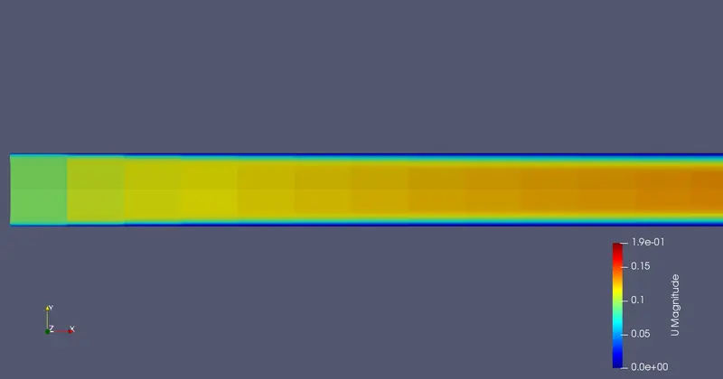
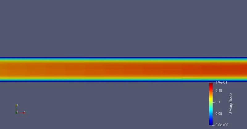
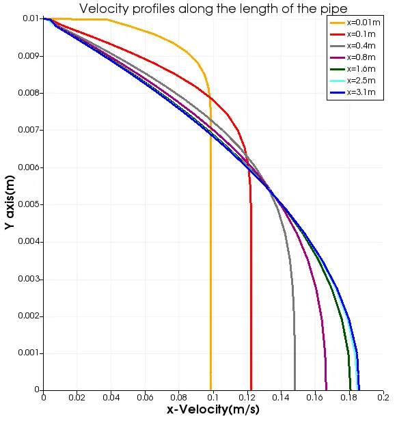
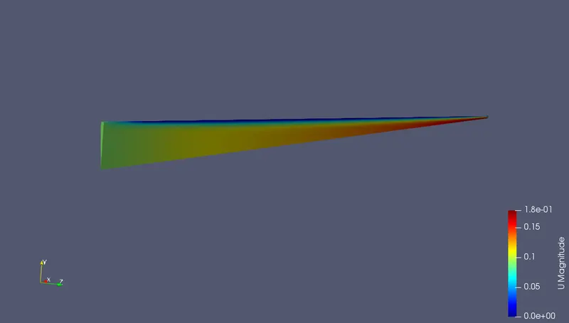
The velocity profile in the below images is perfectly captured with their boundary layer formation from the hydrodynamic entry length all through the end length of the pipe.

WEDGE-SHAPED GEOMETRY:

MIRRORED GEOMETRY:

VELOCITY PROFILES DISTRIBUTION ACROSS THE LENGTH OF THE PIPE:

COMPARISON OF NUMERICAL AND ANALYTICAL VELOCITY PROFILES:

From the equation relating velocity with the length and radius of the pipe which we earlier saw, we frame a graph indicating the velocity profile at x=3.1 meters.

MatLab Code:

clear all
close all
clc
del_p=20.7191;
mu=8.92e-04;
R=0.01;
r=linspace(0,R,20);
l=3.1;
    for j=1:length(r)
        vel(j)=(del_p./(4*mu.*l))*(R^2)*(1-(r(j)^2 ./ R^2));   
    end
figure(1)
plot(vel,r,'linewidth',2,'color','r')
title('Analytical Velocity Profile')
xlabel('x-Velocity')
ylabel('Y-axis(m)')
legend('x=3.1m')
grid on

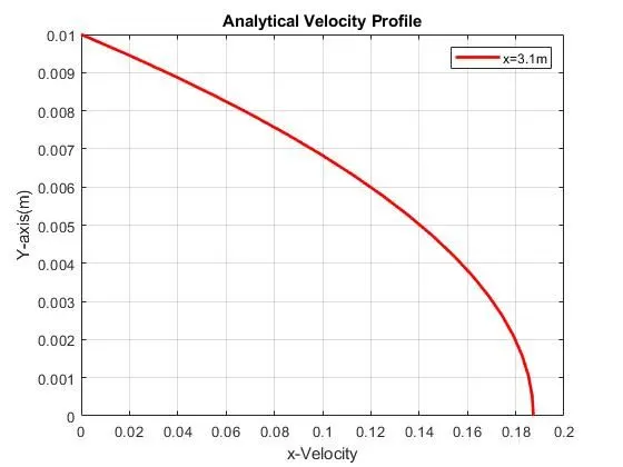
From this graph plot, it is seen that the maximum velocity value obtained from both the numerical and analytical works is almost equal to 0.185 m/s

PRESSURE DISTRIBUTION:

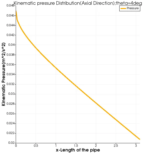
The pressure distribution across the length of the domain is shown in the below image. It seems like it has a greater pressure at the inlet and it eventually decreases leading to pressure loss.

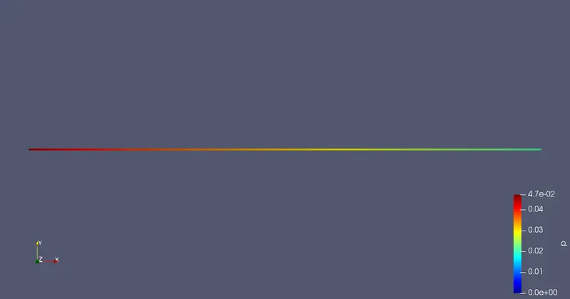
The Kinematic Pressure drop for a 4-degree wedge angle along the length of the entire pipe is shown in the picture below.

SHEAR STRESS DISTRIBUTION:

The image given below clearly shows the initial formation of the boundary layer in the hydrodynamic entry length of the pipe due to shear stress distribution along the radial direction for all the points of the length of the entire pipe.

SHEAR STRESS PROFILES DISTRIBUTION ACROSS THE LENGTH OF THE PIPE:

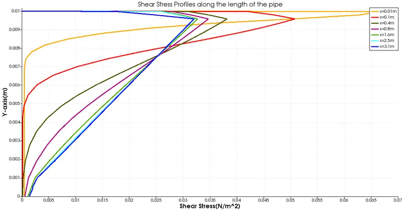
As we saw in the introduction part, the boundary formation is especially due to the presence of shear force between the adjacent layers of fluid. But it eventually becomes lesser as the flow tries to maintain a constant mass flow rate, thus moving with a little higher velocity. Only their magnitude decreases along the length of the pipe, but still, the presence of the shear stress near the walls due to the no-slip condition is unavoidable.

The graph plot obtained from the results of the analysis is an unequivocal evidence of proof for the pre-mentioned inference about the Shear stress in the fluids.