Week 5.1 - Mid term project - Solving the steady and unsteady 2D heat conduction problem
The heat conduction equation in general for a 3-Dimensional case is given as,
(∂T / ∂t) + diffusion *[(∂2T / ∂x2) + (∂2T / ∂y2) + (∂2T / ∂z2)] = 0..............(1)
[(∂2T / ∂x2) + (∂2T / ∂y2) + (∂2T / ∂y2)] = 0..............(2)
wherein,
Equation(1) represents the 3D-Transient heat conduction equation.
Equation(2) represents the 3D-Steady State heat conduction equation.
(∂T / ∂t) - represents the Temperature variation with time(oC/ s), which is a 1st order derivative and is discretized using a Forward Differencing scheme.
diffusion - represents the Thermal diffusivity of the medium(m2 s− 1).
[(∂2T / ∂x2) + (∂2T / ∂y2) + (∂2T / ∂y2)] - represents the spacitial(3D) variation of temperature(oC/m), which are 2nd order derivatives and are generally elliptic type PDEs and thus it is discretized using Central Approximation scheme.
The challenge here requires the analysis and results of the Steady-state and Unsteady (or) Transient 2D heat conduction problem, and thus we reduce the above equations(1 & 2) which is of 3D form into a 2D type equation and are represented in the below equations(3 & 4) where the former is the 2D Transient heat conduction equation and the latter is the 2D Steady-state heat conduction equation.
(∂T / ∂t) + diffusion* [(∂2T / ∂x2) + (∂2T / ∂y2)] = 0..............(3)
[(∂2T / ∂x2) + (∂2T / ∂y2) ] = 0...............(4)
WHAT IS A STEADY-STATE AND AN UNSTEADY STATE HEAT TRANSFER?
The meaning of Steady-state is that the properties measured in any field of space do not vary with respect to time. In general, even after some time(t) the properties in a considered point of interest do not vary and will remain constant throughout the process. This is the basic concept of a steady-state system. So when a system is said to be in a Steady-state condition, then, it is providing a better case to fix the assumption values which makes the calculation better and is also majorly used in Engineering problems and when we see this concept applied in the domain of heat transfer, our region of interest would be in finding the heat transfer across the field to find out its temperature profile.
Heat transfer is the phenomenon that causes the flow of heat energy from the elevated temperature source to the lower temperature side. The modes of heat transfer also can be classified as Conduction, Convection, and Radiation, and here we deal only with conduction. Any system when involving a change in energy within itself due to temperature difference starts as an Unsteady state condition wherein the change in temperature occurs with respect to time. This is because during the start of the process there would be a huge temperature difference between the system and the surroundings due to which it adapts an unsteady or transient condition of heat transfer initially, but later on, when the inlet energy flow and the energy going out (which causes the transient condition) becomes equal, there will be only steady-state heat transfer prevailing inside the system till the end until achieving a Steady-state of the temperature profile, provided there is no external influence of any properties over the system that causes a change in the temperature profile.
The generalized form of the 3D heat conduction equation is given below,
[(∂2T / ∂x2) + (∂2T / ∂y2) + (∂2T / ∂z2)] + (Heat generated/k) = alpha*(∂T / ∂t)................(5)
wherein, the first term of L.H.S represents the inlet and outflow of energy of the considered system and the second term of L.H.S represents the heat generated within the system(mostly avoided during calculations for our ease), and the term in the R.H.S represents the energy change within the system w.r.t time.
ITERATIVE SOLVERS:
In CFD, we may have a set of linear equations which we can solve by two no. of ways (i) Direct method and (ii) Iterative method.
(i) Direct Method: The direct method uses both Gauss-Seidel and Jacobian methods where it can solve a (n x n) matrix with a fixed number of steps. But, this method is inefficient for some engineering problems, since some may have millions of cells forming a huge matrix to solve. Hence for the solving of such kind of huge matrix, the system must require more space. Therefore, the usage of the Direct Method is not a feasible way to get the linear equations solved in CFD.
Thus we go for an aliter for solving such equations, that is by using Iterative Methods.
(ii) Iterative Method: The iterative methods are a better and efficient aliter for the Direct method. Here we will be solving the equations in a way that takes the previously calculated values for a particular grid point at its corresponding time step(for transient condition only) or from its previous time step to calculate the function at that specific point with the help of the reframed governing equations that follows the criterion of different iterative solvers, like,
a) Jacobian Iterative Solver
b) Gauss-Seidel Iterative Solver
c) Successive Over Relaxation Iterative Solver
Of which all the above-mentioned iterative solvers are of Implicit forms. Apart from this, for the Unsteady-state condition, we also do have an explicit form/method to solve the problem statement.
The following flow-chart represents the follow-up of the procedure, how an Iterative solver functions.
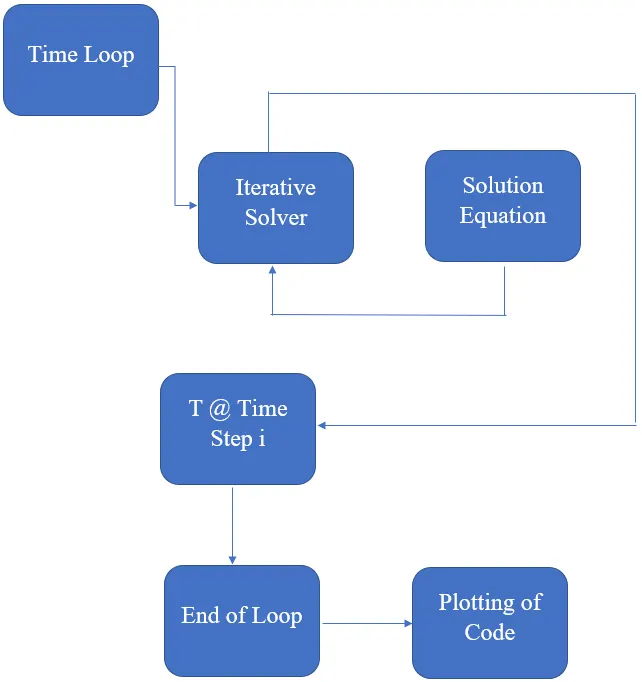
Thus in total, we will be having the following iterative solver types to solve the Conduction analysis problem,
- Implicit form - Steady- State - Jacobian Iterative solver
- Implicit form - Steady- State - Gauss-Seidel Iterative solver
- Implicit form - Steady- State - Successive Over Relaxation Iterative solver(For both Jacobian and Gauss-Seidel Iterative solvers)
- Implicit form - Unsteady- State - Jacobian Iterative solver
- Implicit form - Unsteady- State - Gauss-Seidel Iterative solver
- Implicit form - Unsteady- State - Successive Over Relaxation Iterative solver(For both Jacobian and Gauss-Seidel Iterative solvers)
- Explicit form - Unsteady-State
DIFFERENCE BETWEEN IMPLICIT AND EXPLICIT METHODS:
The solutions for the time-dependent differential equations, either ordinary or partial, are obtained by the numerical analysis, by the numerical approximations done by Implicit or Explicit methods. The explicit form uses the functional values at the previous time-step(n) to calculate the function at the new time-step(n+1) whereas, the implicit form uses the updated values at the time-step(n+1) at each of the previous nodes(i-1) in calculating the functional value at the (n+1) time-step itself for that node(i).
For example, the 1-dimensional linear convection equation which we saw in the last challenge can be taken,
uin+ 1 =uin – c(dt/dx)[ uin – ui-1n]: wherein the right-hand side entirely ha known set of values to calculate the unknown value for the function in its new time step. Thus this is an example of the Explicit form.
uin+ 1 =uin – c(dt/dx)[ uin+1 – ui-1n+1]: whereas, here we have the logical updated values for appropriate nodes on the right-hand side which has the values of the previous nodes for the same time-step for which the function is calculated for. This is an example of the Implicit form.
However, the same concept will be applied in iteration methods, but instead of taking the time steps, we would say that the implicit and explicit forms work with their corresponding iteration step and its previous iteration step respectively.
FUNCTIONS OF DIFFERENT ITERATIVE SOLVERS:
a) Jacobian Iterative Solver: It is one of the types of Iterative solvers, which solves for the diagonal elements of the matrix formed by the linear equations, and the values are approximated in each of the iterations and are just inserted again into the equation until it converges. It generally forms its right-hand side with known values i.e., taking the values from the previous iterations only.
The element-based Jacobian Iterative formula is given as,
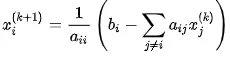 where i - is the nodal number and k - is the iteration step.
b) Gauss-Seidel Iterative Solver: It is also similar to the Jacobian method, and also strictly requires the diagonal matrix for it to perfectly converge. The only difference is that it also forms the right-hand side with values that were just calculated from that corresponding iteration step.
The element-based Gauss-Seidel Iterative formula is given as,
 where i - is the nodal number and k - is the iteration step.
c) Successive Over Relaxation Iterative Solver: This method is used over the Jacobian (or) Gauss-Seidel methods to enhance their results even more quickly with an additional component called Scaling Factor(alpha).
The generalized form of this method is given as,
xik+1 = xik + alpha[(dx/dI)*dI] where i - is the nodal number, k - is the iteration step, alpha- is the Scaling factor and dI is the change in iteration and when relating this generalized equation to the calculated function through the Jacobian and Gauss-Seidel Iterative solvers, we get the equations as
xik+1 = (xik [1-alpha]) + (alpha*TGS) is the SOR over Gauss-Seidel solver.
xik+1 = (xik [1-alpha]) + (alpha*TJac) is the SOR over Jacobian solver.
PROBLEM STATEMENT AND OBJECTIVES:
- To solve the 2D heat conduction equation using the different Iterative solvers and also their implicit and explicit(transient condition only) forms as mentioned above.
- The Boundary conditions for the problem are as follows,
Top Boundary = 600 K
Bottom Boundary = 900 K
Left Boundary = 400 K
Right Boundary = 800 K
- The absolute error criteria is 1e-4.
MATLAB CODE:
MAIN CODE FOR STEADY-STATE CONDITION:
The code given below consists of all the implicit iterative solvers as a function will be called and the results are provided under the corresponding topics.
clear all
close all
clc
%%
%indication of n,x,y terms
n1=input('Enter the number of nodal points(suggestion:enter less than 30 to not exceed the simulation time) : '); %higher the n value, higher is the smoothness and accuracy of the contour;
n2=n1;                                                                     %Indicating the same value for y-axis nodes
x=linspace(0,1,n1);
y=linspace(0,1,n2);
dx=x(2)-x(1);
dy=y(2)-y(1);
[X,Y] = meshgrid(x,y);

%%
%Values for t and its allocations:
T=ones(n1:n2);                                                             %Forming the initial values with a constant value = 1
T(1,:)=900;                                                                %Bottom Boundary Temperature
T(n1,:)=600;                                                               %Top Boundary Temperature
T(:,1)=400;                                                                %Left Boundary Temperature
T(:,n2)=800;                                                               %Right Boundary Temperature
T(1,n1)=(800+900)/2;                                                       %Average Temperature values at the corresponding nodes
T(1,1)=(400+900)/2;
T(n2,1)=(400+600)/2;
T(n2,n1)=(800+600)/2;
T_old=T;                                                                   %Indicating T values to T_old
T_jac=T;                                                                   %Indicating T values to T_jac which will used in SOR over Jacobian.
T_gauss=T;                                                                 %Indicating T values to T_gauss which will used in SOR over Gauss-Seidel.

%%
%Essential data for the iterative solvers
error=9e9;
tol=1e-4;
alpha=1.2;
k=2*((dx^2)+(dy^2))/(dx^2 * dy^2);                                         %(Value of k for Implicit forms of Steady-state-conduction equation)
%k1=(dy^2)/2*((dx^2)+(dy^2));                                              %(Aliter for above coefficient k)k1=1/(k.dx2)
%k2=(dx^2)/2*((dx^2)+(dy^2));                                              %(Aliter for above coefficient k)k1=1/(k.dy2)

%%
%Solution providing different iterative methods:
iterative=input('Enter the type of solver for steady state conduction problem, 1-Jac, 2-Gauss, 3-SOR_Gauss, 4-SOR_Jac : ')


if iterative== 1                                                           %Jacobian Iterative solver
    [T_steady_jac,time_steady_jac,jacob_iter]= steady_jac(n1,n2,k,T_old,T,dx,dy,X,Y,error,tol)
    fprintf('Time taken by the Jacobian Iterative solver to solve = %d seconds.',time_steady_jac);
    fprintf('No. of iterations done to solve the 2D Conduction equation = %d',jacob_iter);
end


if iterative== 2                                                           %Gauss-Seidel Iterative solver
    [T_steady_gauss,time_steady_gauss,gauss_iter]= steady_gauss(n1,n2,k,T_old,T,dx,dy,X,Y,error,tol)
    fprintf('Time taken by the Gauss-Seidel Iterative solver to solve = %d seconds.',time_steady_gauss);
    fprintf('No. of iterations done to solve the 2D Conduction equation = %d',gauss_iter);
end


if iterative== 3                                                           %Successive-Over-Relaxation over GS iterative solver
    [T_steady_sor_gauss,time_steady_sor_gauss,sor_gauss_iter]= steady_sor_gauss(n1,n2,k,T_old,T,dx,dy,X,Y,error,tol,alpha,T_gauss)
    fprintf('Time taken by the SOR_Gauss-Seidel Iterative solver to solve = %d seconds.',time_steady_sor_gauss);
    fprintf('No. of iterations done to solve the 2D Conduction equation = %d',sor_gauss_iter);
end


%Unstable for any values above 1 for alpha
if iterative==4                                                            %Successive-Over-Relaxation over Jacobian iterative solver
    [T_steady_sor_jac,time_steady_sor_jac,sor_jac_iter]= steady_sor_jac(n1,n2,k,T_old,T,dx,dy,X,Y,error,tol,alpha,T_jac)
    fprintf('Time taken by the SOR_Jacobian Iterative solver to solve = %d seconds.',time_steady_sor_jac);
    fprintf('No. of iterations done to solve the 2D Conduction equation = %d',sor_jac_iter);
end
1) Implicit form - Steady- State - Jacobian Iterative solver:
We already knew the 2D steady-state equation represented by equation(4), and we can further reduce it to the nodal form as like,
{(TLEFT -2TP+TRIGHT) / dx2} + {(TBOTTOM - 2TP +TTOP) / dy2} = 0.............(6)
When we further simplify and bring the TP value to L.H.S we may may write the equation as,
Ti,j = (1/k){ Ti+1,j + Ti-1,j / dx2} + (1/k){ Ti,j+1 + Ti,j-1 / dy2}...............(7)
wherein, k=2*( dx2 + dy2) / (dx2 .dy2).........(8)
Thus we know that TP= Ti,j and the corresponding T values in accordance with x and y axes cartesian system and hence we can write the Jacobian form of the Implicit Steady-state equation as,
Tn+1 i,j = (1/k){ Tn i+1,j + Tn i-1,j / dx2} + (1/k){ Tn i,j+1 + Tn i,j-1 / dy2}...........(8)
So as like we have already discussed, the Jacobian method of iteration makes use of the functional values of the previous iteration step to calculate the functional values at the new iteration step.
Note: Here n is the iterative step and i is the nodal number.
The function call CODE for this type of iterative solver is given below,
function [T,time,jacob_iter]= steady_jac(n1,n2,k,T_old,T,dx,dy,X,Y,error,tol)
tic                                                                        %start of simulation time
jacob_iter=1;
while(error>tol)                                                           %Convergence loop
    for i=2:(n1-1)
        for j=2:(n2-1)
            T(i,j)=((1/(k* dx^2))*(T_old(i-1,j)+T_old(i+1,j)))+ ((1/(k* dy^2))*(T_old(i,j+1)+T_old(i,j-1)));
            %T(i,j)=(k1*(T_old(i-1,j)+T_old(i+1,j)))+ (k2*(T_old(i,j+1)+T_old(i,j-1)));
        end
    end
    error=max(max(abs(T-T_old)));                                          %First we are spilitting the matrix into an array by taking the highest values in each of the column and then again max of this array gives the max error value
    jacob_iter=jacob_iter+1;
    T_old=T;
    figure(1)
    [c,d]=contourf(X,Y,T)
    colormap('jet')                                                        %plotting the colormap
    colorbar
    title_text = sprintf('Iteration number=%d for Steady state condition using Jacobian Iterative Solver',jacob_iter);
    title(title_text);
    xlabel('X')
    ylabel('Y')
    clabel(c,d)
    pause(0.03)
end
toc;
time=toc;
end
Results:

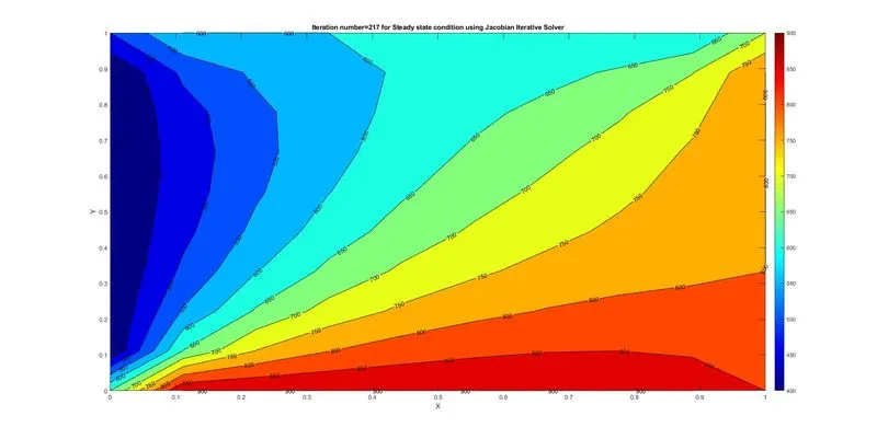

2)Implicit form - Steady- State - Gauss-Seidel Iterative solver:
We can write the reduced Gauss-Seidel form Implicit Steady-state equation as,
Tn+1 i,j = (1/k){ Tn i+1,j + Tn+1 i-1,j / dx2} + (1/k){ Tn i,j+1 + Tn+1 i,j-1 / dy2}..............(9)
wherein in the R.H.S, we consider the updated values of the left(Tn+1 i-1,j ) and bottom node(Tn+1 i,j-1) considering the initial boundary temperatures and the convection direction of temperature over the field. The temperature values at the right(Tn i+1,j) and topside(Tn i,j+1) neighboring nodes are not considered for updated values because those points won't have any kind of updated values since the current iteration has been going on to their previous nodal point i.e., our point of interest(Tn+1 i,j).
Note: Here n is the iterative step and i is the nodal number.
The function call CODE for this type of iterative solver is given below,
function [T,time,gauss_iter]= steady_gauss(n1,n2,k,T_old,T,dx,dy,X,Y,error,tol)
tic                                                                        %start of simulation time
gauss_iter=1;
while(error>tol)                                                           %Convergence loop
    for i=2:(n1-1)
        for j=2:(n2-1)
            T(i,j)=((1/(k* dx^2))*(T(i-1,j)+T(i+1,j)))+ ((1/(k* dy^2))*(T(i,j+1)+T(i,j-1)));
            %T(i,j)=(k1*(T_old(i-1,j)+T_old(i+1,j)))+ (k2*(T_old(i,j+1)+T_old(i,j-1)));
        end
    end
    error=max(max(abs(T-T_old)));                                          %First we are spilitting the matrix into an array by taking the highest values in each of the column and then again max of this array gives the max error value
    gauss_iter=gauss_iter+1;
    T_old=T;
    figure(1)
    [c,d]=contourf(X,Y,T);
    colormap('jet')                                                        %plotting the colormap
    colorbar
    title_text = sprintf('Iteration number=%d for Steady state condition using Gauss-Seidel iterative method',gauss_iter);
    title(title_text);
    clabel(c,d)
    xlabel('X')
    ylabel('Y')
    pause(0.03)
end
toc;
time=toc;
end
Results:

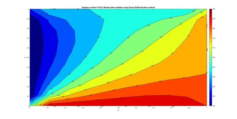

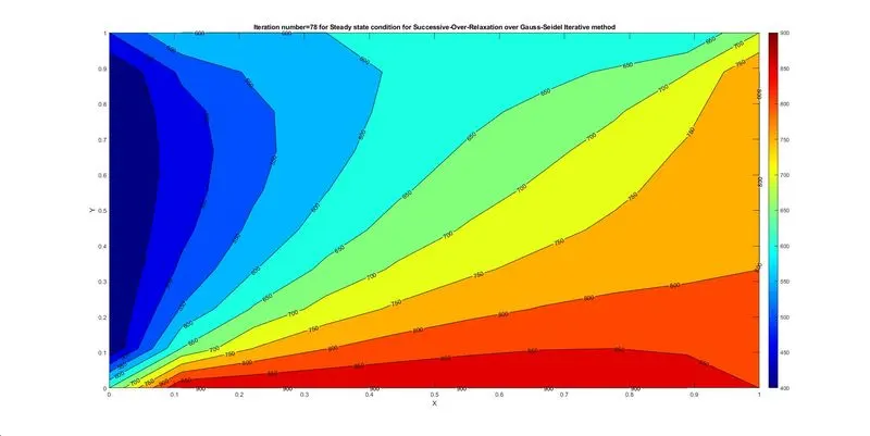
3) Implicit form - Steady- State - Successive Over Relaxation Iterative solver over Gauss-Seidel method:
As we have already seen the basic definition of SOR, which has the purpose to enhance the change encountered in the previous iterative solvers(Jacobian and Gauss-Seidel). Here we take the value of the scaling factor to be 1.2 as it was feasible enough to give a valid result without initial distortion. It can also go up to 1.9 but what happens is that the information surpasses the neighboring node to another node(i+2) which results in distortion or unstableness of the profile and also sometimes causing even more number of iterations to converge.
Tik+1 = (Tik [1-alpha]) + (alpha*TGS)........................(10)
Note: Here k is the iterative step and i is the nodal number.
The function call CODE for this type of iterative solver is given below,
function [T,time,sor_gauss]= steady_sor_gauss(n1,n2,k,T_old,T,dx,dy,X,Y,error,tol,alpha,T_gauss)
    tic                                                                    %start of simulation time
    sor_gauss=1;
    while(error>tol)                                                       %Convergence loop
        for i=2:(n1-1)
            for j=2:(n2-1)
                T(i,j)=((1/(k* dx^2))*(T(i-1,j)+T(i+1,j)))+ ((1/(k* dy^2))*(T(i,j+1)+T(i,j-1)));
                T_gauss=T;
                T(i,j)=((1-alpha)*T_old(i,j)) + (alpha* T_gauss(i,j));
            end
        end
        error=max(max(abs(T-T_old)));                                      %First we are spilitting the matrix into an array by taking the highest values in each of the column and then again max of this array gives the max error value
        sor_gauss=sor_gauss+1;
        T_old=T;

        figure(1)
        [c,d]=contourf(X,Y,T);
        colormap('jet')                                                    %plotting the colormap
        colorbar
        title_text = sprintf('Iteration number=%d for Steady state condition for Successive-Over-Relaxation over Gauss-Seidel Iterative method',sor_gauss);
        title(title_text);
        clabel(c,d)
        xlabel('X')
        ylabel('Y')
        pause(0.03)
    end
    toc;
    time=toc;
end
Results:


4) Implicit form - Steady- State - Successive Over Relaxation Iterative solver over Jacobian method:
Similarly, we can also use SOR over the previously used Jacobian iterative solver.
xik+1 = (xik [1-alpha]) + (alpha*TJac)................(11)
Note: Here k is the iterative step and i is the nodal number where alpha value was taken as 1.2
The function call CODE for this type of iterative solver is given below,
function [T,time,sor_jac]= steady_sor_jac(n1,n2,k,T_old,T,dx,dy,X,Y,error,tol,alpha,T_jac)
tic
sor_jac=1;
    while(error>tol)
        for i=2:(n1-1)
            for j=2:(n2-1)
                T(i,j)=((1/(k* dx^2))*(T_old(i-1,j)+T_old(i+1,j)))+ ((1/(k* dy^2))*(T_old(i,j+1)+T_old(i,j-1)));
                T_jac=T;
                T(i,j)=((1-alpha)*T_old(i,j)) + (alpha* T_jac(i,j));
            end
        end
        error=max(max(abs(T-T_old)));
        sor_jac=sor_jac+1;
        T_old=T;
        figure(1)
        [c,d]=contourf(X,Y,T);
        colormap('jet')
        colorbar
        title_text = sprintf('Iteration number=%d for Steady state condition for Successive-Over-Relaxation over Jacobian Iterative method',sor_jac);
        title(title_text);
        clabel(c,d)
        xlabel('X')
        ylabel('Y')
        pause(0.03)
    end
    toc;
    time=toc;
end
Results:
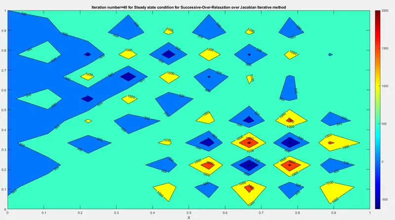
Generally, the Steady-state condition follows an Implicit form approach, which is mostly stable at all times, but within which the usage of SOR(Successive Over Relaxation) method over Jacobian Iterative solver brings Unstableness to the solution.
The sole purpose for which we use the SOR method is to get a quicker convergence by using the scaling factor value of more than 1, but the SOR_Jacobian Iterative solver fails with its stability when we use the scaling factor value more than 1. Thus we avoid using this method because the information surpasses the neighboring nodal point and creates rippleness in the result leading to instability.

MAIN CODE FOR UNSTEADY (OR) TRANSIENT STATE CONDITION:
The code given below consists of all the implicit iterative solvers and an explicit solver as a function will be called and the results are provided under the corresponding topics.
clear all
close all
clc
%%
%indication of n,x,y terms
n1=input('Enter the number of nodal points(suggestion:enter less than 30 to not exceed the simulation time) : '); %higher the n value, higher is the smoothness and accuracy of the contour;
n2=n1;                                                                     %Indicating the same value for y-axis nodes
x=linspace(0,1,n1);
y=linspace(0,1,n2);
dx=x(2)-x(1);
dy=y(2)-y(1);

%%
%Values for t and its allocations:
T=300*ones(n1:n2);                                                         %Forming the initial values with a constant value = 1
T(1,:)=900;                                                                %Bottom Boundary Temperature
T(n1,:)=600;                                                               %Top Boundary Temperature
T(:,1)=400;                                                                %Left Boundary Temperature
T(:,n2)=800;                                                               %Right Boundary Temperature
T(1,n1)=(800+900)/2;                                                       %Average Temperature values at the corresponding nodes
T(1,1)=(400+900)/2;
T(n2,1)=(400+600)/2;
T(n2,n1)=(800+600)/2;
T_old=T;                                                                   %Indicating T values to T_old
T_initial=T_old;                                                           %Indicating T_old or T values to T_initial which is used for each iteration for time loop.
T_gauss=T;                                                                 %Indicating T values to T_jac which will used in SOR over Gauss-Seidel.
T_jac=T;                                                                   %Indicating T values to T_jac which will used in SOR over Jacobian.

%%
%Essential data for the iterative solvers
error=9e9;
tol=1e-4;                                                                  %absolute error criterion
diff=1.4;                                                                  %diffusion term  %As this value increases we may need increased simulation time for convergence
dt=1e-3;                                                                   %time interval dt
alpha=1.2;                                                                 %Scaling factor
k1= diff * (dt/ dx^2);
k2= diff * (dt/ dy^2);
term1=(1+ 2*k1 + 2*k2)^-1;
term2=k1*term1;
term3=k2*term1;

%%
%Solution providing different iterative methods:
%Implicit forms:
iterative=input('Enter the type of solver for steady state conduction problem, 1-Jac, 2-Gauss, 3-SOR_Gauss, 4-SOR_Jac, 5-Explicit : ')

if iterative==1                                                            %Jacobian Iterative solver
    jac_iter=1
    [T_transient_jac,time_transient_jac,jacob_iter]=transient_jac(n1,n2,T_old,T_initial,T,dx,dy,x,y,tol,term1,term2,term3,jac_iter)
    fprintf('Time taken by the Jacobian Iterative solver to solve = %d seconds.',time_transient_jac);
    fprintf(' No. of iterations done to solve the 2D Conduction equation = %d',jacob_iter);
end

if iterative==2                                                            %Gauss-Seidel Iterative solver
    gauss_iter=1;
    [T_transient_gauss,time_transient_gauss,gauss_iter]=transient_gauss(n1,n2,T_old,T_initial,T,dx,dy,x,y,tol,term1,term2,term3,gauss_iter)
    fprintf('Time taken by the Gauss-Seidel Iterative solver to solve = %d seconds.',time_transient_gauss);
    fprintf(' No. of iterations done to solve the 2D Conduction equation = %d',gauss_iter);
end

if iterative==3                                                            %Successive-Over-Relaxation over GS iterative solver
    sor_gauss_iter=1;
    [T_transient_sor_gauss,time_transient_sor_gauss,sor_gauss_iter]=transient_sor_gauss(n1,n2,T_old,T_initial,T,x,y,tol,term1,term2,term3,alpha,sor_gauss_iter)
    fprintf('Time taken by the SOR_Gauss-Seidel Iterative solver to solve = %d seconds.',time_transient_sor_gauss);
    fprintf(' No. of iterations done to solve the 2D Conduction equation = %d',sor_gauss_iter);
end

if iterative==4                                                            %Successive-Over-Relaxation over Jacobian iterative solver
    sor_jac_iter=1;
    [T_transient_sor_jac,time_transient_sor_jac,sor_jac_iter]=transient_sor_jac(n1,n2,T_old,T_initial,T,x,y,tol,term1,term2,term3,alpha,sor_jac_iter)
    fprintf('Time taken by the SOR_Jacobian Iterative solver to solve = %d seconds.',time_transient_sor_jac);
    fprintf(' No. of iterations done to solve the 2D Conduction equation = %d',sor_jac_iter);
end


if iterative==5                                                            %Explicit form of unsteady state conduction
    exp_iter=1;
    [T_transient_explicit,time_transient_explicit,explicit_iter]=transient_explicit(n1,n2,T_old,T_initial,T,x,y,tol,k1,k2,exp_iter)
    fprintf('Time taken by the Iterative Explicit solver to solve = %d seconds.',time_transient_explicit);
    fprintf(' No. of iterations done to solve the 2D Conduction equation = %d',explicit_iter);
end
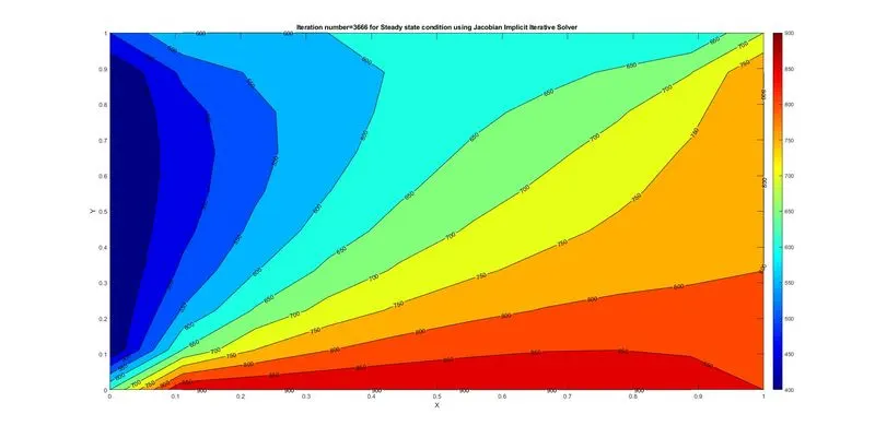
5) Implicit form - Unsteady- State - Jacobian Iterative solver:
We already knew the 2D steady-state equation represented by equation(4), and we can further reduce it to the nodal form as like,
(∂T / ∂t) + alpha *[{(TLEFT -2TP+TRIGHT) / dx2} + {(TBOTTOM - 2TP +TTOP) / dy2}] = 0.............(12)
When we further simplify and bring the TP value to L.H.S we may write the equation as,
Tn+1 i,j = [Tn i,j + {k1 * (Tn i+1,j + Tn i-1,j)} + {k2 * (Tn i,j+1 + Tn i,j-1 )}] / (1 + 2k1 + 2k2)................(13)
where k1 = Diffusiion * dt / dx2and is also called as the x-CFL number.
k1 = Diffusiion * dt / dy2and is also called as the y-CFL number.
The CFL condition states that the sum of x-CFL and y-CFL together when it is greater than 0.5, then the results may go unstable. This CFL is also referred to as the Stability criterion and must be given almost importance while selecting the terms it is comprised of.
Thus this instead state too follows the same Jacobian method as discussed for the steady-state but the only change involved here is the updation of the functional values for every iteration for each time-step for which we employ a Time loop inside which we keep the convergence loop, and the functional values are updated within the time step and outside the convergence loop and then again fed back to the same convergence loop in order to move the profile with a transient state
The function call CODE for this type of iterative solver is given below,
function [T,time,jac_iter]=transient_jac(n1,n2,T_old,T_initial,T,dx,dy,x,y,tol,term1,term2,term3,jac_iter)
tic                                                                        %start of simulation time

for p=1:1400                                                               %time loop
    error=9e9
    while(error>tol)                                                       %convergence loop
            for i=2:(n1-1)
                for j=2:(n2-1)
                    H=(T_old(i-1,j) + T_old(i+1,j));
                    V=(T_old(i,j-1) + T_old(i,j+1));
                    T(i,j)= (term1*T_initial(i,j)) + (term2*H) + (term3*V);

                end
            end

            error=max(max(abs(T-T_old)));                                  %First we are spilitting the matrix into an array by taking the highest values in each of the column and then again max of this array gives the max error value
            T_old=T;                                                       %Upddating the values after each iteration
            jac_iter=jac_iter+1;

    end
             T_initial = T;                                                %updating the value after each time step
            figure(1)
            [c,d]=contourf(x,y,T);
            colormap('jet');                                               %plotting the colormap
            colorbar;
            clabel(c,d);
            title_text = sprintf('Iteration number=%d for Steady state condition using Jacobian Implicit Iterative Solver',jac_iter);
            title(title_text);
            xlabel('X')
            ylabel('Y')
            pause(0.03)

    end
    toc;                                                                   %end time of simulation
    time=toc;
end
Results:


6) Implicit form - Unsteady- State - Gauss-Seidel Iterative solver:
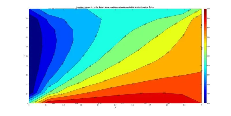
Similar to the above Jacobian iteration, the Gauss-Seidel type of iteration follows only a small change in the governing equation with the consideration of functional values from previous nodes of the same iteration step.
Tn+1 i,j = [Tn i,j + {k1 * (Tn i+1,j + Tn+1 i-1,j)} + {k2 * (Tn i,j+1 + Tn+1 i,j-1 )}] / (1 + 2k1 + 2k2)................(13)
where k1 = Diffusiion * dt / dx2and is also called as the x-CFL number.
k1 = Diffusiion * dt / dy2and is also called as the y-CFL number.
The function call CODE for this type of iterative solver is given below,
function [T,time,gauss_iter]= transient_gauss(n1,n2,T_old,T_initial,T,dx,dy,x,y,tol,term1,term2,term3,gauss_iter)
tic                                                                        %start of simulation time


for p=1:1400                                                               %time loop
    error=9e9;
    while(error>tol)                                                       %convergence loop


            for i=2:(n1-1)
                for j=2:(n2-1)
                    H=(T(i-1,j) + T_old(i+1,j));
                    V=(T(i,j-1) + T_old(i,j+1));
                    T(i,j)= (term1*T_initial(i,j)) + (term2*H) + (term3*V);

                end
            end

            error=max(max(abs(T-T_old)));                                  %First we are spilitting the matrix into an array by taking the highest values in each of the column and then again max of this array gives the max error value
            T_old=T;                                                       %Upddating the values after each iteration
            gauss_iter=gauss_iter+1;
    end
            T_initial = T;                                                 %updating the value after each time step
            figure(1)
            [c,d]=contourf(x,y,T);
            colormap('jet');                                               %plotting the colormap
            colorbar;
            clabel(c,d)
            title_text = sprintf('Iteration number=%d for Steady state condition using Gauss-Seidel Implicit Iterative Solver',gauss_iter);
            title(title_text);
            xlabel('X')
            ylabel('Y')
            pause(0.03)

    end
    toc;                                                                   %end time of simulation
    time=toc;
end
Results:


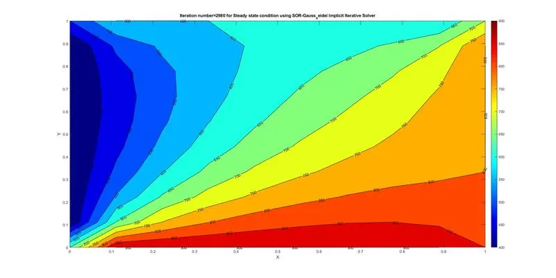
7) Implicit form - Unsteady- State - Successive Over Relaxation Iterative solver over Gauss-Seidel method:
As we have already seen the SOR over Jacobian and Gauss-seidel iterative solver for steady-state.
The usage of it over the Unsteady also does not differ very much and is still the same, but the only difference is that we must use the updated values within the convergence loop i.e., T_old, and should not use the updated values for each time step i.e., T_initial.
xik+1 = (xik [1-alpha]) + (alpha*Tgauss)................(11)
Note: Here k is the iterative step and i is the nodal number where alpha value was taken as 1.2
The function call CODE for this type of iterative solver is given below,
function [T,time,sor_gauss_iter]= transient_sor_gauss(n1,n2,T_old,T_initial,T,x,y,tol,term1,term2,term3,alpha,sor_gauss_iter)
tic                                                                        %start of simulation time

    for p=1:1400                                                           %time loop
        error=9e9
    while(error>tol)                                                       %convergence loop


            for i=2:(n1-1)
                for j=2:(n2-1)
                    H=(T(i-1,j) + T_old(i+1,j));
                    V=(T(i,j-1) + T_old(i,j+1));
                    T(i,j)= (term1*T_initial(i,j)) + (term2*H) + (term3*V);
                    T_gauss=T;
                    T(i,j)=((1-alpha)*T_old(i,j)) + (alpha* T_gauss(i,j));

                end
            end

            error=max(max(abs(T-T_old)));                                  %First we are spilitting the matrix into an array by taking the highest values in each of the column and then again max of this array gives the max error value
            T_old=T;                                                       %Upddating the values after each iteration
            sor_gauss_iter=sor_gauss_iter+1;

    end
            T_initial = T;                                                 %updating the value after each time step
            figure(1)
            [c,d]=contourf(x,y,T);
            colormap('jet');                                               %plotting the colormap
            colorbar;
            clabel(c,d)
            title_text = sprintf('Iteration number=%d for Steady state condition using SOR-Gauss_seidel Implicit Iterative Solver',sor_gauss_iter);
            title(title_text);
            xlabel('X')
            ylabel('Y')
            pause(0.03)

    end
    toc;                                                                   %end time of simulation
    time=toc;
end
Results:


8) Implicit form - Unsteady- State - Successive Over Relaxation Iterative solver over Jacob method:
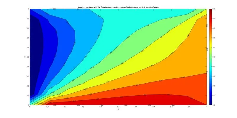
Similarly, for the case of the Jacobian method as the previous one.
xik+1 = (xik [1-alpha]) + (alpha*TJacob)................(12)
Note: Here k is the iterative step and i is the nodal number where alpha value was taken as 1.2
The function call CODE for this type of iterative solver is given below,
function [T,time,sor_jac_iter]=transient_sor_jac(n1,n2,T_old,T_initial,T,x,y,tol,term1,term2,term3,alpha,sor_jac_iter)
tic                                                                        %start of simulation time
    for p=1:1400                                                           %time loop
        error=9e9;
    while(error>tol)                                                       %convergence loop


            for i=2:(n1-1)
                for j=2:(n2-1)
                    H=(T_old(i-1,j) + T_old(i+1,j));
                    V=(T_old(i,j-1) + T_old(i,j+1));
                    T(i,j)= (term1*T_initial(i,j)) + (term2*H) + (term3*V);
                    T_jac=T;
                    T(i,j)=((1-alpha)*T_old(i,j)) + (alpha* T_jac(i,j));

                end
            end

            error=max(max(abs(T-T_old)));                                  %First we are spilitting the matrix into an array by taking the highest values in each of the column and then again max of this array gives the max error value
            T_old=T;                                                       %Upddating the values after each iteration
            sor_jac_iter=sor_jac_iter+1;
    end
            T_initial = T;                                                 %updating the value after each time step
            figure(1)
            [c,d]=contourf(x,y,T);
            colormap('jet');                                               %plotting the colormap
            colorbar;
            clabel(c,d)
            title_text = sprintf('Iteration number=%d for Steady state condition using SOR-Jacobian Implicit Iterative Solver',sor_jac_iter);
            title(title_text);
            xlabel('X')
            ylabel('Y')
            pause(0.03)

    end
    toc;                                                                   %end time of simulation
    time=toc;
end
Results:


9) Explicit form - Unsteady-State:
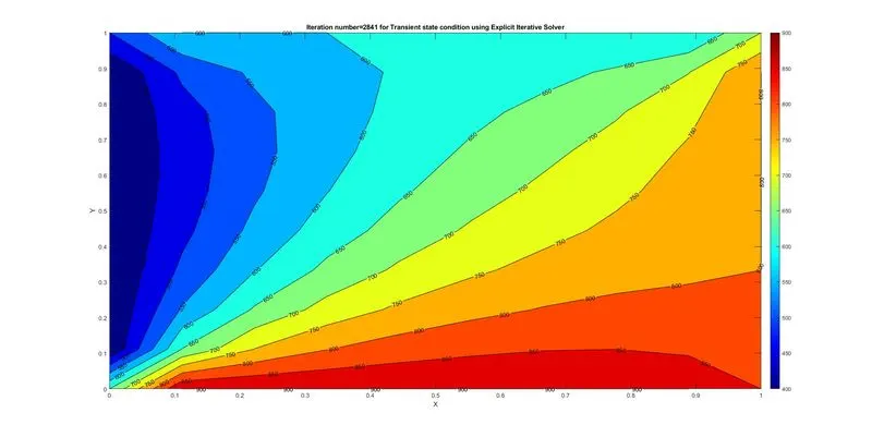
The explicit form differs from the reframed implicit governing equation wherein the other terms remain the same. The governing equation for this explicit form Unsteady problem is given by,
Tn+1 i,j = [Tn i,j + {k1 * (Tn i+1,j - 2Tni,j + Tn i-1,j)} + {k2 * (Tn i,j+1 - 2Tni,j + Tn i,j-1 )}]............(13)
k1 = Diffusiion * dt / dx2and is also called as the x-CFL number.
k1 = Diffusiion * dt / dy2and is also called as the y-CFL number.
The function call CODE for this type of iterative solver is given below,
function [T,time,exp_iter]=transient__explicit_1(n1,n2,T_old,T_initial,T,X,Y,tol,k1,k2,exp_iter)
tic                                                                        %start of simulation time

    for p=1:1400                                                           %time loop
        error=9e9;
        while(error>tol)                                                   %convergence loop


            for i=2:(n1-1)
                for j=2:(n2-1)
                    H=(T_old(i-1,j) - 2*T_old(i,j) + T_old(i+1,j));
                    V=(T_old(i,j-1) - 2*T_old(i,j) + T_old(i,j+1));
                    T(i,j)= T_initial(i,j) + (k1*H) + (k2*V);

                end
            end

            error=max(max(abs(T-T_old)));                                  %First we are spilitting the matrix into an array by taking the highest values in each of the column and then again max of this array gives the max error value
            T_old=T;                                                       %Upddating the values after each iteration
            exp_iter=exp_iter+1;

         end
            T_initial = T;                                                 %updating the value after each time step
            figure(1)
            [c,d]=contourf(X,Y,T);
            colormap('jet');                                               %plotting the colormap
            colorbar;
            clabel(c,d);
            title_text = sprintf('Iteration number=%d for Transient state condition using Explicit Iterative Solver',exp_iter);
            title(title_text);
            xlabel('X')
            ylabel('Y')
            pause(0.03)

    end
    toc;                                                                   %end time of simulation
    time=toc;
end
Results:


RESULTS AND CONCLUSION:
| ITERATIVE SOLVER TYPE | NO. OF ITERATIONS | SIMULATION TIME(seconds) |
| Implicit form - Steady State -Jacobian Iterative solver | 217 | 34.18 |
| Implicit form - Steady State -Gauss-Seidel Iterative solver | 116 | 16.61 |
| Implicit form - Steady State-SOR Gauss-Seidel Iterative solver | 78 | 12.04 |
| Implicit form - Steady State-SOR Jacobian Iterative solver | ---(Unstable) | ---(Unstable) |
| Implicit form - Unsteady State -Jacobian Iterative solver | 3666 | 213.154 |
| Implicit form - Unsteady State -Gauss-Seidel Iterative solver | 3114 | 255.66 |
| Implicit form - Unsteady State-SOR Gauss-Seidel Iterative solver | 2980 | 239.81 |
| Implicit form - Unsteady State-SOR Jacobian Iterative solver | 3037 | 208.91 |
| Explicit form - Unsteady State | 2841 | 217.70 |
- From the above observation, we could see that for the steady-state condition, we assume that the system is in a perfectly balanced condition in terms of its energy and only a steady flow prevails till the end of the process. Thus it takes very little time and iterates its values for a little number of steps to reach the steady-state.
- We also knew that the unsteady state condition prevails for all the problems where there is a huge difference in the temperature margin either within the system or its surroundings. Thus it will take some time to find a steady path to balance the energy within the system and hence it requires more time than the time taken for the steady-state condition.
- Also, when we look at the Iterative solvers, the most efficient way is to use the SOR method but it also has some demerits which we have previously observed. However, it takes the first place for its efficient way of converging the results with lesser iterations.
- The following is the order of efficiency for the iterative solvers for both Steady and Unsteady state heat conduction.
Steady State : Imp_SOR_Gauss > Imp_Gauss > Imp_Jacobian
Unsteady State : Explicit > Imp_SOR_Gauss > Imp_SOR_Jac > Imp_Gauss > Imp_Jacobian
- The Simulation time is just a rough approximation done to get the idea of how much time was the iteration done to converge, but it is a system-operated one and often may not be true.