Week 7 - Simulation of a 1D Super-sonic nozzle flow simulation using Macormack Method

Aim:

To investigate steady-state flow-field variables of both the conservative and non-conservative forms of the governing equations viz. continuity, momentum and energy equation, and to compare these two forms by comparing their solutions.

Theory:

We consider the steady, isentropic flow through a convergent-divergent nozzle as sketched in Fig. 1, shown below,

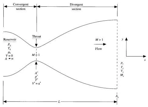
There are three zones viz. convergent section, throat, divergent section, through which fluid flows. The flow-field variables such as pressure, temperature, density, velocity, mach number, at inlet, throat and outlet, are shown in above figure.

We assume that at a given section, where the cross-sectional area is A, the flow properties are uniform across that section. Hence, although the area of the nozzle changes as a function of distance along the nozzle, x, and therefore in reality the flow field is two-dimensional (the flow varies in the two-dimensional xy space), we make the assumption that the flow properties vary only with x; this is tantamount to assuming uniform flow properties across any given cross section. Such flow is defined as quasi-one-dimensional flow.

The governing equations for quasi-one-dimensional flow through convergent-divergent nozzle, are given in two forms, viz. Conservative form and Non-conservative form. These two forms are given as follows,

1.1 Conservative form of governing equations

#Continuity equation

`(del(rhoA))/(delt)+(del(rhoAV))/(delx)=0`(Eq. 1)

#Momentum equation

`(del(rhoAV))/(delt)+(del(rhoAV^2))/(delx)=-(delP)/(delx)` (Eq. 2)

#Energy equation

`(del(rhoV^2/2A))/(delt)+(del(rhoV^3/2A))/(delx)=-AV(delP)/(delx)` (Eq. 3)

1.2 Non-conservative form of governing equations

#Continuity equation

`(del(rhoA))/(delt)+V(del(rhoA))/(delx)=-rhoA(delV)/(delx)` (Eq. 4)

#Momentum equation

`rho(delV)/(delt)+pV(delV)/(delx)=-(delP)/(delx)` (Eq. 5)

#Energy equation

`rho(dele)/(delt)+rhoV(dele)/(delx)=-P(delV)/(delx)-rhoV(del(lnA))/(delx)` (Eq. 6)

For nozzle flows, the flow-field variables are frequently expressed in terms of nondimensional variables. The nondimensional variables `p/p_0` , `rho/rho_0` , and `T/T_0`vary between 0 and 1, which is an aesthetic advantage when presenting the results. The nondimensional variables are given as follows,

`T^'=T/T_0`, `rho^'=rho/rho_0`, `x^'=x/L`, `V^'=V/a_0=V/sqrt(gammaRT_0`, `t^'=t/(L/a_0)`, `A^'=A/A^**`

1.3 Non-dimensionalised conservative form of governing equations

Continuity equation, `(del(rho^'A^'))/(delt^')+(del(rho^'A^'V^'))/(delx^')=0` (Eq. 7)

Momentum equation, `(del(rho^'A^'V^'))/(delt^')+(del(rho^'A^'(V^')^2+(1/gamma)P^'A^'))/(delx)=(1/gamma)P^'(delA^')/(delx^')` (Eq. 8)

Energy equation, `(del(rho^'(e^'/(gamma-1)+gamma/2(V^')^2)A^'))/(delt^')+(del(rho^'(e^'/(gamma-1)+gamma/2(V^')^2)V^'A^'+P^'A^'V^'))/(delx^')` (Eq. 9)

1.4 Non-dimensionalised non-conservative form of governing equations

Continuity equation, `(delrho^')/(delt^')=-rho^'(delV^')/(delx^')-rho^'V^'(del(lnA^'))/(delx^')-V^'(delrho^')/(delx)` (Eq. 10)

Momentum equation, `(delV^')/(delt^')=-V^'(delV^')/(delx^')-1/gamma((delT^')/(delx^')+T^'/rho^'(delP^')/(delx))` (Eq. 11)

Energy equation, `(delT^')/(delt^')=-V^'(delT^')/(delx^')-(gamma-1)T^'((delV^')/(delx^')+V^'(del(lnA^'))/(delx^'))` (Eq. 12)

Above partial differential equations can be solved by following steps such as meshing, discredizing and solving.

1.5 Meshing

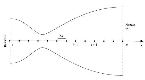
As given in above figure, we can divide length of nozzle into number of nodes. As we are following one dimensional flow, we can consider `Deltax` as the distance between consecutive nodes.

1.6 Discretization

Here, we can use Mac-cormack's technique.

1.6.1 For non-conservative form of governing equations,

It's LHS can be solved by time-marching solution and RHS can be solved by forward/backward differencing solution. The steps to be followed, are,

Step 1: Initial conditions

`rho=1-0.3146x`

`T=1-0.2314x`

`V=(0.1+1.09x)T^(1/2)`

`A=1+2.2(x-1.5)^2`

Step 2: Predictor step

Here, 'f' is any flow-field variable. The partial derivative of 'f' with respect to time is calculated i.e. `(delf)/(delt_p)` such that, the modified equations are as follows,

Continuity equation, `((rho_i^(n+1)-rho_i^n)/(Deltat))_p=-rho_i^n((V_(i+1)^n-V_i^n)/(Deltax))-rho_i^nV_i^n((lnA_(i+1)^n-lnA_i^n)/(Deltax))-V_i^n((rho_(i+1)^n-rho_i^n)/(Deltax))` (Eq. 13)

where, `f_i^n` denotes value of flow-field variable at 'i'th node and 'n' th time step.

We can write, `((delV)/(delx))_(FD)^n=(V_(i+1)^n-V_i^n)/(Deltax)`

`((del(lnA))/(delx))_(FD)^n=(lnA_(i+1)^n-lnA_i^n)/(Deltax)`

`((delrho)/(delx))_(FD)^n=(rho_(i+1)^n-rho_i^n)/(Deltax)`

`((delT)/(delx))_(FD)^n=(T_(i+1)^n-T_i^n)/(Deltax)`

`((delP)/(delx))_(FD)^n=(P_(i+1)^n-P_i^n)/(Deltax)`

So, momentum equation can be written as,

`((V_i^(n+1)-V_i^n)/(Deltat))_p=-V((delV)/(delx))_(FD)^n-1/gamma(((delT)/(delx))_(FD)^n+T^'/rho^'((delP)/(delx))_(FD)^n)` (Eq. 14)

Similarly, energy equation can be written as,

`((T_(i+1)^n-T_i^n)/(Deltat))_p=-V((delT)/(delx))_(FD)^n-(gamma-1)T(((delV)/(delx))_(FD)^n+V((del(lnA))/(delx))_(FD)^n)` (Eq. 15)

Step 3: Solution update

The values calculated from previous step i.e. `((delf)/(delt))_p` , are used in following formula,

`f^n=f_(Ini)+((delf)/(delt))_p*Deltat`

Here, `f_(Ini)` is value at initial condition. `Deltat` is time step. This is calculated by following method.

`(Deltat)_i^t=C*(Deltax)/(sqrt(T_i^t)+V_i^t`

where, 'C' is Courant number(here C=0.5). For i=1 to i=n, one has to calculate `(Deltat)_i^t` and then choose the minimum value.

`Deltat=min(Deltat_1^t,Deltat_2^t,....,Deltat_i^t,....,Deltat_n^t)`

Step 4: Corrector step

Here, 'f' is any flow-field variable. The partial derivative of 'f' with respect to time is calculated i.e. `((delf)/(delt))_c`. The procedure is almost same as that of predictor step except for the calculation of flow-field derivative terms. Here, backword differencing method is used.

`((delV)/(delx))_(BD)^n=(V_(i)^n-V_(i-1)^n)/(Deltax)`

`((del(lnA))/(delx))_(BD)^n=(lnA_(i)^n-lnA_(i-1)^n)/(Deltax)`

`((delrho)/(delx))_(BD)^n=(rho_(i)^n-rho_(i-1)^n)/(Deltax)`

`((delT)/(delx))_(BD)^n=(T_(i)^n-T_(i-1)^n)/(Deltax)`

`((delP)/(delx))_(BD)^n=(P_(i)^n-P_(i-1)^n)/(Deltax)`

Step 5: Average of predictor and corrector step

`((delf)/(delt))_(avg)=0.5*(((delf)/(delt))_p+((delf)/(delt))_c)`

Step 6: Final solution update

`f^(n+1)=f_(Ini)+((delf)/(delt))_(avg)*Deltat`

1.6.2 For conservative form of governing equations,

Initial conditions,

For `0lexle0.5`

`rho=1.0`

`T=1.0`

For `0.5lexle1.5`

`rho=1-0.366(x-0.5)`

`T=1-0.167(x-0.5)`

For `1.5lexle3.5`

`rho=0.634-0.3879(x-1.5)`

`T=0.833-0.3507(x-1.5)`

The steps are same as that of previous form but there are some substitutions in governing equations. (Eq. 7, 8, 9)

`U_1=rho^'A^'`

`U_2=rho^'A^'V^'`

`U_3=rho^'(e^'/(gamma-1)+gamma/2(V^')^2)A^'`

`F_1=rho^'A^'V^'=U_2`

`F_2=rho^'A^'(V^')^2+(1/gamma)P^'A^'=U_2^2/U_1+(gamma-1)/gamma(U_3-gamma/2U_2^2/U_1)`

`F_3=rho^'(e^'/(gamma-1)+gamma/2(V^')^2)V^'A^'+P^'A^'V^'=gamma(U_2U_3)/U_1-(gamma(gamma-1))/2U_2^3/U_1^2`

`J_2=(1/gamma)P^'(delA^')/(delx^')=(gamma-1)/gamma(U_3-gamma/2U_2^2/U_1)(del(lnA))/(delx)`

After calculating `U_1, U_2, U_3` , one can find primitive variables by using following method,

`rho^'=U_1/A^'`

`V^'=U_2/U_1`

`T^'=e^'=(gamma-1)(U_3/U_1-gamma/2(V^')^2)`

`P^'=rho^'T^'`

1.7 Solving

For non-conservative form of governing equations,

Boundary conditions,

At inlet, `V_1=2V_2-V_3`

At outlet, `V_n=2V_(n-1)-V_(n-2)`

`rho_n=2rho_(n-1)-rho_(n-2)`

`T_n=2T_(n-1)-T_(n-2)`

For conservative form of governing equations,

Boundary conditions,

At inlet, `U_1=A_(i=1)^'`

`U_(2(i=1))=2U_(2(i=2))-U_(2(i=3))`

`U_3=U_1(T^'/(gamma-1)+gamma/2(V^')^2)`

At outlet, `(U_1)_n=2(U_1)_(n-1)-(U_1)_(n-2)`

`(U_2)_n=2(U_2)_(n-1)-(U_2)_(n-2)`

`(U_3)_n=2(U_3)_(n-1)-(U_3)_(n-2)`

Objectives:

• To plot steady-state distribution of primitive variables inside the nozzle
• To plot time-wise variation of the primitive variables
• To plot variation of mass flow rate distribution inside the nozzle at different time steps during the time-marching process
• To compare normalized mass flow rate distributions of both forms
• To perform a grid independence test on the solution

MATLAB code:

#Main code

close all
clear all
clc

%Inputs
L=3;
n=[31 62 93];
nt=[1:1000];

for i=1:length(n)
x=linspace(0,L,n(i));
[mfr_nc,mfr_nc_node]=nozzle_flow_1D_nonconservative(n(i));
[mfr_c,mfr_c_node]=nozzle_flow_1D_conservative(n(i));
figure(7)
subplot(2,1,1)
plot(nt,mfr_nc,'b',nt,mfr_c,'r')
xlabel('Time steps, nt')
ylabel('Mass flow rate')
legend('Non-conservative form','Conservative form')
title('Comparison between Non-conservative and conservative form - Mass flow rate(w.r.t. nt')
subplot(2,1,2)
plot(x,mfr_nc_node,'b',x,mfr_c_node,'r')
xlabel('Length of nozzle, x')
ylabel('Mass flow rate')
legend('Non-conservative form','Conservative form')
title('Comparison between Non-conservative and conservative form - Mass flow rate(w.r.t. x')
figure(8)
subplot(2,1,1)
hold on
plot(nt,mfr_nc)
xlabel('Time steps, nt')
ylabel('Mass flow rate')
legend('at n=31','at n=62','at n=93')
title('Grid independency test: Non-conservative form')
subplot(2,1,2)
hold on
plot(nt,mfr_c)
xlabel('Time steps, nt')
ylabel('Mass flow rate')
legend('at n=31','at n=62','at n=93')
title('Grid independency test: Conservative form')
end

This main code contains functions of two forms viz. Conservative and non-conservating form of governing equations. Inputs are length of computational domain, L, set of number of nodes for checking mesh indepedence, n, and number of time steps for attaining steady state, nt.

To get different plots for grid independence test, 'for' loop is used. To compare the solutions of both forms, one needs any of the flow-field variable, here mass flow rate is taken. Functions of these forms give two outputs. One is for the mass flow rate at specific node for number of time steps i.e. mfr_c/mfr_nc and other is for the mass flow rate at every nodes for the length of nozzle i.e. mfr_c_node/mfr_nc_node. Also, one can check the grid independency by observing a specific node for different number of nodes. 'subplot' command let user to add multiple plots in a single window.

#Function for non-conservative form of governing equation

function [mfr_nc,mfr_nc_node]=nozzle_flow_1D_nonconservative(n)

%Inputs
L=3;
x=linspace(0,L,n);
dx=L/(n-1);

%Initial condition
rho=1-0.3146.*x;
t=1-0.2314.*x;
v=(0.1+1.09.*x).*t.^0.5;
a=1+2.2.*((x-1.5).^2);
gamma=1.4;

Here, inputs are same as discussed earlier. Initial conditions are discussed in theory section 1.6.1 for both forms.

%CFL condition
CFL=0.5;
nt=linspace(0,1000,1000);

Generally, the CFL condition for 1D PDE is `CFLle1`. But to more accurate results, here CFL is taken as 0.5. An array is used for time steps.

%Time loop
for l=1:length(nt)
    rho_old=rho;
    t_old=t;
    v_old=v;
    for i=1:n
        d_t(i)=CFL*dx/(sqrt(t(i))+v(i));
    end
    dt=min(d_t);
    %Predictor method
    for i=2:n-1
        drhodx_p=(rho(i+1)-rho(i))/dx;
        dvdx_p=(v(i+1)-v(i))/dx;
        dlogadx_p=(log(a(i+1))-log(a(i)))/dx;
        dtdx_p=(t(i+1)-t(i))/dx;
        %Continuity equation
        drhodt_p(i)=-rho(i)*dvdx_p-rho(i)*v(i)*dlogadx_p-v(i)*drhodx_p;
        %Momentum equation
        dvdt_p(i)=-v(i)*dvdx_p-(1/gamma)*(dtdx_p+(t(i)/rho(i))*drhodx_p);
        %Energy equation
        dtdt_p(i)=-v(i)*dtdx_p-(gamma-1)*t(i)*(dvdx_p+(v(i)*dlogadx_p));
        
        %Solution update
        rho(i)=rho(i)+drhodt_p(i)*dt;
        v(i)=v(i)+dvdt_p(i)*dt;
        t(i)=t(i)+dtdt_p(i)*dt;
    end

Initial values of flow-field variables are saved as rho_old, t_old, v_old. As discussed in theory (section 1.6.1), the minimun time step is taken for further calculation. In predictor method, all steps are taken as discussed in theory (section 1.6.1). At the end of the loop, solution update is there.

 %Corrector method
    for i=2:n-1
        drhodx_c=(rho(i)-rho(i-1))/dx;
        dvdx_c=(v(i)-v(i-1))/dx;
        dlogadx_c=(log(a(i))-log(a(i-1)))/dx;
        dtdx_c=(t(i)-t(i-1))/dx;
        %Continuity equation
        drhodt_c(i)=-rho(i)*dvdx_c-rho(i)*v(i)*dlogadx_c-v(i)*drhodx_c;
        %Momentum equation
        dvdt_c(i)=-v(i)*dvdx_c-(gamma^-1)*(dtdx_c+(t(i)/rho(i))*drhodx_c);
        %Energy equation
        dtdt_c(i)=-v(i)*dtdx_c-(gamma-1)*t(i)*(dvdx_c+(v(i)*dlogadx_c));
    end

Steps are taken as per the theory discussed in section 1.6.1.

%Average
    drhodt_avg=0.5*(drhodt_p+drhodt_c);
    dvdt_avg=0.5*(dvdt_p+dvdt_c);
    dtdt_avg=0.5*(dtdt_p+dtdt_c);

Here, average of both predictor and corrector steps, is taken.

%Final solution
    for k=2:n-1
        rho(k)=rho_old(k)+drhodt_avg(k)*dt;
        v(k)=v_old(k)+dvdt_avg(k)*dt;
        t(k)=t_old(k)+dtdt_avg(k)*dt;
    end

The old values and average of partial derivatives of flow-field variables are used here.

%Apply the boundary conditions
    %Inlet
    v(1)=2*v(2)-v(3);
    %Outlet
    v(n)=2*v(n-1)-v(n-2);
    rho(n)=2*rho(n-1)-rho(n-2);
    t(n)=2*t(n-1)-t(n-2);

Here, boundary conditions are applied.

for i=1:n
        p(i)=rho(i).*t(i);
        M(i)=v(i)./sqrt(t(i));
        mfr(i)=rho(i).*a(i).*v(i);
    end

Other flow-field variables are calculated from `rho, V, T`, which are pressure, mach number and mass flow rate.

if n==31
        for ll=[1 50:100:600 700];
            if l==ll
                figure(1)
                hold on
                plot(x,mfr)
                xlabel('Length of nozzle')
                ylabel('Mass flow rate')
                title('Non-conservative form: Variation of Mass flow rate distribution inside the nozzle at different time steps during the time-marching process')
            elseif l==1000
                plot(x,mfr,'*r')
                legend('at time step 1','at time step 50','at time step 150','at time step 250','at time step 350','at time step 450','at time step 550','at time step 700','at time step 1000')
            end
        end
end

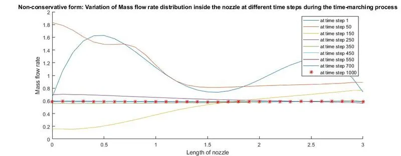
Here, variation of mass flow rate distribution inside the nozzle at different time steps during the time-marching process, is plotted. Some time steps values out of 1000, are selected to show in plot.

    rho_at_node(l)=rho(16);
    v_at_node(l)=v(16);
    t_at_node(l)=t(16);
    p_at_node(l)=p(16);
    M_at_node(l)=M(16);
    mfr_at_node(l)=mfr(16);
end

Here, values of flow-field variables at i=16, are calculated for every time loop.

if n==31
    figure(2)
    plot(nt,rho_at_node,'g',nt,v_at_node,'b',nt,t_at_node,'r',nt,p_at_node,'y',nt,M_at_node,'m',nt,mfr_at_node,'c')
    xlabel('Time step, nt')
    ylabel('Non-dimentional variables')
    title('Non-conservative form: Time-wise variation of the primitive variables at a node')
    legend('Density','Velocity','Temperature','Pressure','Mach number','Mass flow rate')
    figure(3)
    plot(x,rho,'g',x,v,'b',x,t,'r',x,p,'y',x,M,'m',x,mfr,'c')
    xlabel('Length of nozzle, x')
    ylabel('Non-dimentional variables')
    title('Non-conservative form: Steady-state distribution of primitive variables inside the nozzle')
    legend('Density','Velocity','Temperature','Pressure','Mach number','Mass flow rate')
    title(sprintf('Time step = %d',l))
end
mfr_nc=mfr_at_node;
mfr_nc_node=mfr;
end

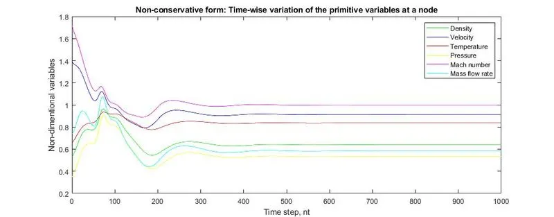
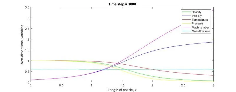
These are the plots for 'Time-wise variation of the primitive variables at a node' and 'Steady-state distribution of primitive variables inside the nozzle' for number of nodes,n, is 31. This function gives 'mfr_nc' and 'mfr_nc_node' as output.

#Function for conservative form of governing equation

function [mfr_c,mfr_c_node]=nozzle_flow_1D_conservative(n)
%Inputs
L=3;
x=linspace(0,L,n);
dx=L/(n-1);
gamma=1.4;

%Initial condition
for i=1:length(x)
    if x(i)<=0.5 && x(i)>=0
        rho(i)=1;
        t(i)=1;
    end
end
for i=1:length(x)
    if x(i)<=1.5 && x(i)>=0.5
        rho(i)=1-0.366*(x(i)-0.5);
        t(i)=1-0.167*(x(i)-0.5);
    end
end
for i=1:length(x)
    if x(i)<=3 && x(i)>=1.5
        rho(i)=0.634-0.3879*(x(i)-1.5);
        t(i)=0.833-0.3507*(x(i)-1.5);
    end
end
for i=1:length(x)
    a(i)=1+2.2.*((x(i)-1.5).^2);
    v(i)=0.59/(rho(i)*a(i));
end
%Initialization of solution vector
u1=rho.*a;
u2=rho.*a.*v;
u3=rho.*((t/(gamma-1))+(0.5*gamma.*(v.^2))).*a;

%Initialization of flux vector
f1=u2;
f2=((u2.^2)./u1)+((gamma-1)/gamma).*(u3-(0.5*gamma.*((u2.^2)./u1)));
f3=gamma.*((u2.*u3)./u1)-(0.5*gamma*(gamma-1).*((u2.^3)/(u1.^2)));

Here, inputs are same as that for previous case. Initial conditions are as per the theory discussed in section 1.6.2.

%CFL condition
CFL=0.5;
nt=linspace(0,1000,1000);

for l=1:length(nt)
    u1_old=u1;
    u2_old=u2;
    u3_old=u3;
    for i=1:n
        d_t(i)=CFL*dx/(sqrt(t(i))+v(i));
    end
    dt=min(d_t);
    %Predictor method
    for i=2:n-1
        df1dx_p=(f1(i+1)-f1(i))/dx;
        df2dx_p=(f2(i+1)-f2(i))/dx;
        df3dx_p=(f3(i+1)-f3(i))/dx;
        dlogadx_p=(log(a(i+1))-log(a(i)))/dx;
        j2_p=((gamma-1)/gamma).*(u3-(0.5*gamma*((u2.^2)./u1))).*dlogadx_p;
        %Continuity Equation
        du1dt_p(i)=-df1dx_p;
        %Momentum equation
        du2dt_p(i)=-df2dx_p+j2_p(i);
        %Energy equation
        du3dt_p(i)=-df3dx_p;
        %Solution update
        u1(i)=u1(i)+du1dt_p(i)*dt;
        u2(i)=u2(i)+du2dt_p(i)*dt;
        u3(i)=u3(i)+du3dt_p(i)*dt;
        f1(i)=u2(i);
        f2(i)=((u2(i).^2)./u1(i))+((gamma-1)/gamma).*(u3(i)-(0.5*gamma.*((u2(i).^2)./u1(i))));
        f3(i)=gamma.*((u2(i).*u3(i))./u1(i))-(0.5*gamma*(gamma-1).*((u2(i).^3)/(u1(i).^2)));
    end
    %Corrector method
    for i=2:n-1
        df1dx_c=(f1(i)-f1(i-1))/dx;
        df2dx_c=(f2(i)-f2(i-1))/dx;
        df3dx_c=(f3(i)-f3(i-1))/dx;
        dlogadx_c=(log(a(i))-log(a(i-1)))/dx;
        j2_c=((gamma-1)/gamma).*(u3-(0.5*gamma*((u2.^2)./u1))).*dlogadx_c;
        %Continuity Equation
        du1dt_c(i)=-df1dx_c;
        %Momentum equation
        du2dt_c(i)=-df2dx_c+j2_c(i);
        %Energy equation
        du3dt_c(i)=-df3dx_c;
    end
    %Average
    du1dt_avg=0.5*(du1dt_p+du1dt_c);
    du2dt_avg=0.5*(du2dt_p+du2dt_c);
    du3dt_avg=0.5*(du3dt_p+du3dt_c);

Here, instead of taking density, velocity and tempearture(RHS in previous case) , u1, u2, u3 are defined and LHS comprises of f1, f2, f3 and j2. 'f' denotes flux vector and 'j' denotes source term. The remaining procedure is same as that of previous case.

    %Final solution
    for k=2:n-1
        u1(k)=u1_old(k)+du1dt_avg(k)*dt;
        u2(k)=u2_old(k)+du2dt_avg(k)*dt;
        u3(k)=u3_old(k)+du3dt_avg(k)*dt;
    end
    
    %Apply the boundary conditions
    %Inlet
    %u1=rho*a as at i=1, rho=1, so u1=a
    u1(1)=a(1);
    u2(1)=2*u2(2)-u2(3);
    u3(1)=u1(1)*((t(1)/(gamma-1))+(0.5*gamma.*(v(1).^2)));
    %Outlet
    u1(n)=2*u1(n-1)-u1(n-2);
    u2(n)=2*u2(n-1)-u2(n-2);
    u3(n)=2*u3(n-1)-u3(n-2);
    for i=1:n
        f1(i)=u2(i);
        f2(i)=((u2(i).^2)./u1(i))+((gamma-1)/gamma).*(u3(i)-(0.5*gamma.*((u2(i).^2)./u1(i))));
        f3(i)=gamma.*((u2(i).*u3(i))./u1(i))-(0.5*gamma*(gamma-1).*((u2(i).^3)/(u1(i).^2)));
    end

Here, final solution is calculated. Boundary conditions are applied as per discussed in theory(sec. 1.7). At the end of this loop, flux vectors are updated.

    %Primitive variables
    rho=u1./a;
    v=u2./u1;
    t=(gamma-1).*((u3./u1)-(0.5*gamma.*(v.^2)));
    p=rho.*t;
    M=v./sqrt(t);
    mfr=rho.*a.*v;

Primitive variables are calculated from u1, u2, and u3 as discussed in theory (section 1.6.2).

    if n==31
        for ll=[1 50:100:600 700];
            if l==ll
                figure(4)
                hold on
                plot(x,mfr)
                xlabel('Length of nozzle')
                ylabel('Mass flow rate')
                title('Conservative form: Variation of Mass flow rate distribution inside the nozzle at different time steps during the time-marching process')
            elseif l==1000
                plot(x,mfr,'*r')
                legend('at time step 1','at time step 50','at time step 150','at time step 250','at time step 350','at time step 450','at time step 550','at time step 700','at time step 1000')
            end
        end
    end

Here, variation of mass flow rate distribution inside the nozzle at different time steps during the time-marching process, is plotted. Some time steps values out of 1000, are selected to show in plot.

    rho_at_node(l)=rho(16);
    v_at_node(l)=v(16);
    t_at_node(l)=t(16);
    p_at_node(l)=p(16);
    M_at_node(l)=M(16);
    mfr_at_node(l)=mfr(16);
end

Here, values of flow-field variables at i=16, are calculated for every time loop.

if n==31
    figure(5)
    plot(nt,rho_at_node,'g',nt,v_at_node,'b',nt,t_at_node,'r',nt,p_at_node,'y',nt,M_at_node,'m',nt,mfr_at_node,'c')
    xlabel('Time step, nt')
    ylabel('Non-dimentional variables')
    title('Conservative form: Time-wise variation of the primitive variables at a node')
    legend('Density','Velocity','Temperature','Pressure','Mach number','Mass flow rate')
    figure(6)
    plot(x,rho,'g',x,v,'b',x,t,'r',x,p,'y',x,M,'m',x,mfr,'c')
    xlabel('Length of nozzle, x')
    ylabel('Non-dimentional variables')
    title('Conservative form: Steady-state distribution of primitive variables inside the nozzle')
    legend('Density','Velocity','Temperature','Pressure','Mach number','Mass flow rate')
    title(sprintf('Time step = %d',l))
end
mfr_c=mfr_at_node;
mfr_c_node=mfr;
end

These are the plots for 'Time-wise variation of the primitive variables at a node' and 'Steady-state distribution of primitive variables inside the nozzle' for number of nodes,n, is 31. This function gives 'mfr_c' and 'mfr_c_node' as output.

Outputs:

#Variation of Mass flow rate distribution inside the nozzle at different time steps during the time-marching process

For non-conservative form of governing equation

For conservative form of governing equation

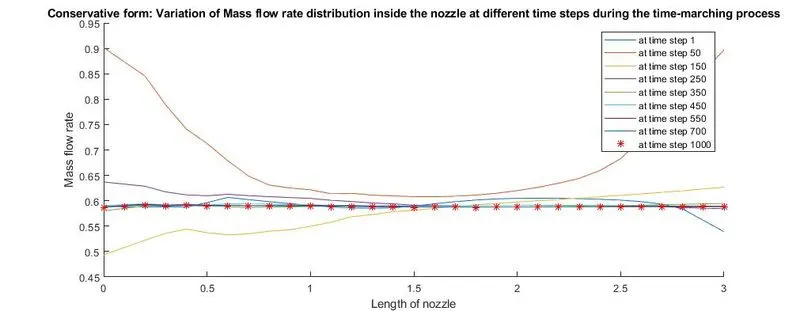
• Comparing both plots, one can infer that both forms tend to give steady state solution with mass flow rate between 0.55 and 0.6.
• Conservative form starts to converge earlier than that of non-conservative form.
• Also, initial values of conservative form are more close to steady-state solution.

#Time-wise variation of the primitive variables

For non-conservative form of governing equation

For conservative form of governing equation

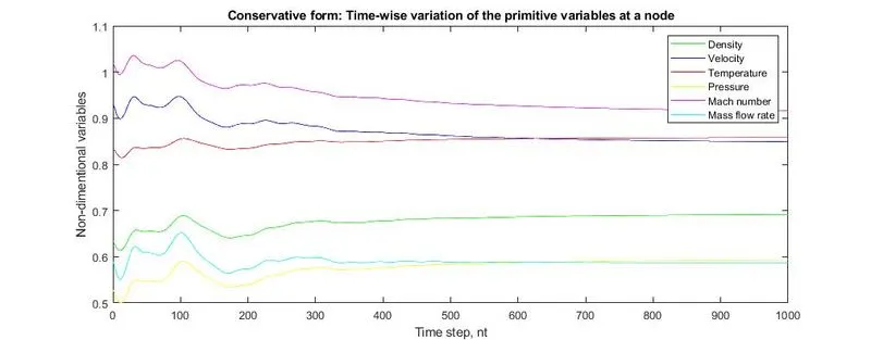
• One can infer that the non-conservative form achieves steady-state a little early inspite large variations in consecutive time steps. Conservative form at `nt~~520` and non-conservative form at `nt~~480`.
• Intial guess for conservative form is more accurate than that of non-conservative form.

#Steady-state distribution of primitive variables inside the nozzle

For non-conservative form of governing equation

For conservative form of governing equation

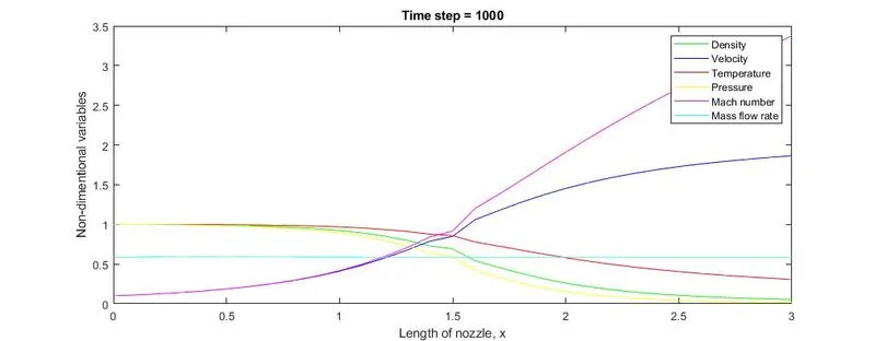
• These plots show values of flow-field variables at the end of time step=1000.
• If we consider velocity,then one can see initially, the velocity is below sound velocity (i.e. subsonic). At throat area (`x~~1.5`), its value is 1(i.e. sonic) and after that it increases continuously(i.e. supersonic).

#Comparison between conservative and non-conservative forms with respect to mass flow rate

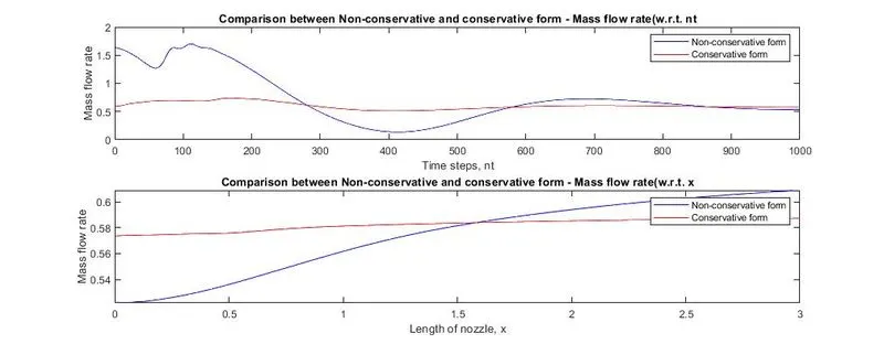
• Both forms reach the stable and exact solution by the end of time steps. But the rate of convergence is more with respect to conservative form than non-conservative forn.
• When we compare both form with respect to the length of nozzle, for the conservative form, the mass flow rate is stable (i.e. `dotm~~0.57`). On other hand, for non-conservative form, it's mass flow rate fluctuates between 0.54 and 0.6.
• Though the stability is attained at lesser time steps, the computational time is more in case of conservative form.

#Grid Independence Test

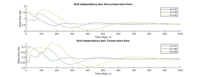
• Though values of mass flow rate for different number of grid points, are different initially. But over the period of time, all of them achieve steady state at almost same number of time steps (`nt~~600`).