Week 4.1 - Genetic Algorithm
Aim:
To undertand the concept of genetic algorithm, stalagmite function and ways to optimise the stalagmite function. Also, to write a code in MATLAB that will optimise the stalagmite function using 'ga' command and its attributes.
Governing equations:
Stalagmite function,
`f(x,y)=f_(1,x)*f_(2,x)*f_(1,y)*f_(2,y)`
where,
`f_(1,x)=(sin(5.1*pi*x+0.5))^6`
`f_(1,y)=(sin(5.1*pi*y+0.5))^6`
`f_(2,x)=exp(-4*ln(2)*((x-0.0667)^2)/0.64)`
`f_(2,y)=exp(-4*ln(2)*((y-0.0667)^2)/0.64)`
Objectives:
- To study about how the genetic algorithm works and 'ga' syntax used in MATLAB
- To study the optimization of stalagmite function in MATLAB using different 'ga' options
- To plot unbounded and bounded region of stalagmite function which gives different local maximas
- To find global maxima of stalagmite function
Theory:
Genetic algorithm
Genetic algorithm developed by Goldberg was inspired by Darwin's theory of evolution which states that the survival of an organism is affected by rule "the strongest species that survives". Darwin also stated that the survival of an organism can be maintained through the process of reproduction, crossover and mutation. This theory is then adopted to computational algorithm, which determines the solution of objective function. Here, the objective function is 'Stalagmite function'. These solution will undergo a process called fitness function to measure the suitability of solution generated by GA with problem. Consecutively, this collection of solutions i.e. Population, is given a fitness score. As the algorithm progresses, these fitness scores get scaled up. These are called expectation values. Based on these expectation values, parents are selected and the process of reproduction, crossover and mutation happen until one of the stopping criteria is met.
Mutation is making random changes to a single parent and Crossover is by combining the vector entries of a pair of parents.
Some of the stopping criteria are as follows,
-
MaxGenerations - The algorithm stops when the number of generations reaches MaxGenerations.
-
MaxTime - The algorithm stops after running for an amount of time in seconds equal to MaxTime.
-
FitnessLimit - The algorithm stops when the value of the fitness function for the best point in the current population is less than or equal to FitnessLimit.
-
MaxStallGenerations - The algorithm stops when the average relative change in the fitness function value over MaxStallGenerations is less than FunctionTolerence.
-
MaxStallTime - The algorithm stops if there is no improvement in the objective function during an interval of time in seconds equal to MaxStallTime.
- FunctionTolerance - The algorithm runs until the average relative change in the fitness function value over MaxStallGenerations is less than FunctionTolerance.
Syntax for 'ga'
The basic syntax is x=ga(fun,nvars), which gives local unconstrained minimum, x of an objective function, fun and 'nvars' are number of design variables.
In this project, following syntax are used,
[x, fval]=ga(fun,nvars)
This gives additional value i.e. 'fval' value of function. All others are same as basic syntax.
[x, fval]=ga(fun,nvars,A,b,Aeq,beq,lb,ub)
Here, A,b and Aeq,beq are coefficients of linear inequalities and linear equalities respectively. lb, ub are lower bound and upper bound respectively which are useful in constraining the local minimum.
[x, fval]=ga(fun.nvars,A,b,Aeq,beq,lb,ub,nonlcon,options)
Addition to previous syntax, 'nonlcon' subjects the minimization to the constraints defined in nonlcon. 'options' minimizes 'ga' with the default optimization parameters replaced by values in options. This includes various optimization options, out of which 'PopulationSize' is what we require.
MATLAB Code:
#Defining search space
x=linspace(0,0.6,150);
y=linspace(0,0.6,150);
num_cases=45;
Here, we are creating a search space to run the genetic algorithm. So. 'linspace' command creates 150 values in the range 0 to 0.6. Also, we are defining 'num_cases' as 45 which limits number of generations.
[xx yy]=meshgrid(x,y);This command generates 2D array of x and y values.
#'for' loop for assigning x and y values to stalagmite function
for i= 1:length(xx)
    for j=1:length(yy)
        input_vector(1)=xx(i,j);
        input_vector(2)=yy(i,j);
        f(i,j)=stalagmite(input_vector);
    end
end
Here, we are assigning x and y values to an array called 'input_vector'. This array can be input to the stalagmite function. The code for stalagmite function is as follows,
function [func_xy]=stalagmite(input_vector)
f_1_x=(sin(((5.1*pi).*input_vector(1))+0.5)).^6;
f_1_y=(sin(((5.1*pi).*input_vector(2))+0.5)).^6;
f_2_x=exp(-4*log(2)*(((input_vector(1)-0.0667).^2)/0.64));
f_2_y=exp(-4*log(2)*(((input_vector(2)-0.0667).^2)/0.64));
func_xy = -((f_1_x)*(f_1_y)*(f_2_x)*(f_2_y));
end
Here, we are assigning minus sign(-) to the output of stalagmite function. This is due to the fact that the 'ga' command gives local minima but our aim is to find local maxima. The equations are input(discussed in theory section) in this code.
#'for' loop to solve stalagmite function using genetic algorithm
Case 1: Defining number of iterations to constrain the maximum number of generation
tic
%Evaluating a stalagmite function
for i= 1:num_cases
   [inputs, f_opt(i)]=ga(@stalagmite,2);
    x_opt(i)=inputs(1);
    y_opt(i)=inputs(2);
end
cs_time_1=toc
Here, tic_toc command is used to measure time required to go through the code. 'i' is loop counter variable which runs the code till length of num_cases i.e. 45 times. Also, the basic syntax of 'ga' is used. The solutions are saved in 'inputs' and local maximum So it gives large number of local maximas. Out of that, global maxima is difficult to calculate. So, this is called as an unbounded solution or unbounded population.
Case 2: Defining lower and upper bound to constrain function maxima within search space
for i= 1:num_cases
   [inputs, f_opt(i)]=ga(@stalagmite,2,[],[],[],[],[0;0],[1;1]);
    x_opt(i)=inputs(1);
    y_opt(i)=inputs(2);
end
Here, in 'ga' syntax, one can define upper and lower bound. So, lower bound is [0;0] and upper bound is [1;1]. This gives a bounded solution or bounded population.
Case 3: Defining PopulationSize to constrain the solution within limited population
options=optimoptions('ga')
options=optimoptions(options,'PopulationSize',260);
tic
for i= 1:num_cases
   [inputs, f_opt(i)]=ga(@stalagmite,2,[],[],[],[],[0;0],[0.6;0.6],[],[],options);
    x_opt(i)=inputs(1);
    y_opt(i)=inputs(2);
end
'options' uses optimization parameters such as 'PopulationSize' to limit the population growth. Here, 'PopulationSize' is set as 260. Also, comparing with previous case, here, upper bound is reduced to [0.6,0.6]. This further limits the scope, so one can get global maxima.
#Plotting
figure(1)
subplot(2,1,1)
surfc(xx,yy,-f)
shading interp
hold on
plot3(x_opt,y_opt,-f_opt,'marker','o','markersize',5,'markerfacecolor','r')
xlabel('X-axis')
ylabel('Y-axis')
zlabel('F maximum')
title('Unbounded inputs')
subplot(2,1,2)
plot(-f_opt)
xlabel('Iterations')
ylabel('Function maximum')
display(inputs)
figure(1) opens a new window with plot. In the same window, one can show two plots or more than two plots by using 'subplot' command. 'surfc' generates 3D plot with stalagmites in which different local maximas are shown. 'shading interp' command smooths the surface by removing points mesh. 'plot3' generates 3D co-ordinate system, in which 'x_opt', 'y_opt' and '-f_opt' are plotted. 'title' can be changed as per the case. Also, second subplot comprises of 'F maximum Vs. No. of iterations'.
Output of the code:
#Case 1: Unbounded solution or population
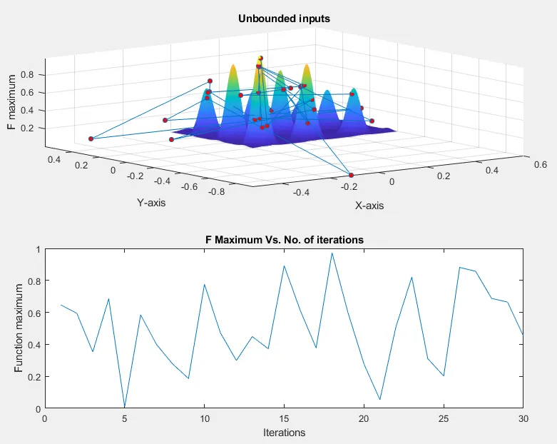
Here, there are large number of local maximas both within search space and out of search space. This solution does not give global maxima. So, the code is to be refined more to get constrained solution. So, we go for case 2.
#Case 2: Bounded solution or population with pre-defined Lower and Upper boundary
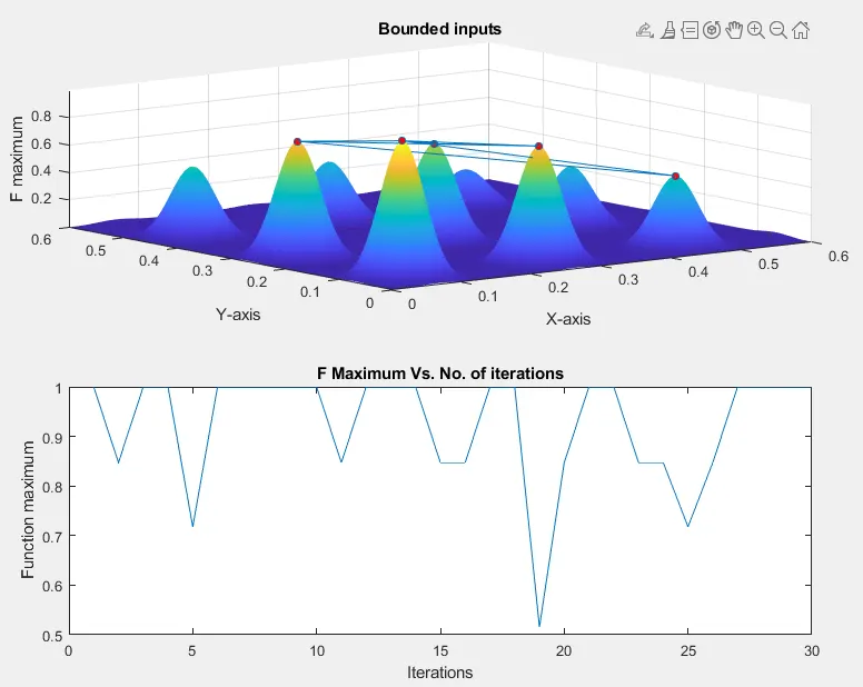
This plot is more resolved than previous one. But still there are few number of local maximas. We want to know the global maxima of stalagmite function. The number of iterations for both cases is same. This can be further refined by defining population size and increasing number of iterations. So, we go for case 3.
#Case 3: Bounded solution or population with defined population size and increased number of iterations
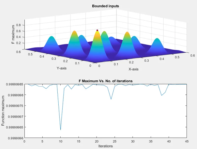
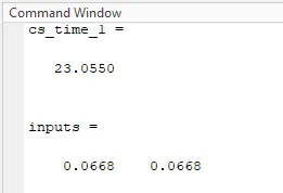
This case gives the global maxima as shown in above plot. This is the desired solution. The values of x and y co-ordinates for which this code gives maximum function value, are as follows,
Errors:
#Error 1
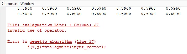
This error was coming due to wrong coding of stalagmite function. The position of element operator was wrong.
#Error 2
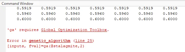
Earlier, I had not installed an extension to MATLAB i.e. Global Optimization Toolbox. So, after installing that, the error was resolved.
Conclusion:
Different optimization techniques explained above, give refined solution than prior case. So, it is important to use different options in 'ga' command. So, when we constrain boundaries of solution as well as as population size, we get optimum solution that gives global maxima of any objective function.
References: