Challenge

Project 1 - Parsing NASA thermodynamic data

YYash Gujarathi27 Jun 2021

Aim:

To analyse the data from NASA thermodynaic data file and to evaluate molecular weights of species and it's thermodynamic properties such as Cp, H and S with respect to temperature range, by using MATLAB Program.

Governing Equations:

NASA came up with polynomials that can be used to evaluate thermodynamic properties such as Cp, H and S. They have also documented the co-efficients that are required to evaluate these polynomials for 1000+ species. The polynomials for Cp, H and S are as follows,

Here, a1, a2, a3, a4, a5, a6, a7 are high temperature (above 1000K) coefficients and a8, a9, a10, a11, a12, a13, a14 are low temperature (below 1000K) coefficients. The 'THERMO.dat' file consists of these 14 coefficients defined for differernt species. Each species is having different local temperature ranges.

Objectives:

To write a function that extracts the 14 co-efficients and calculates the enthalpy, entropy and specific heats for all the species in the data file
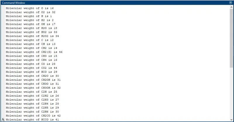
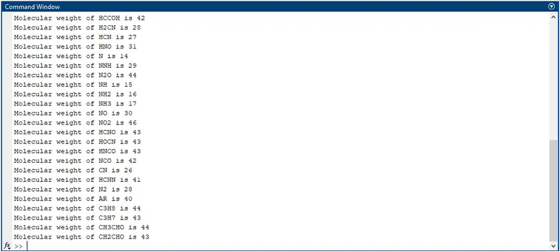
To calculate the molecular weight of each species and display it in the command window
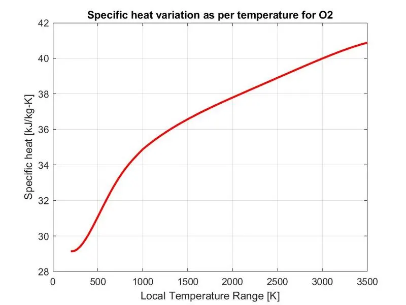
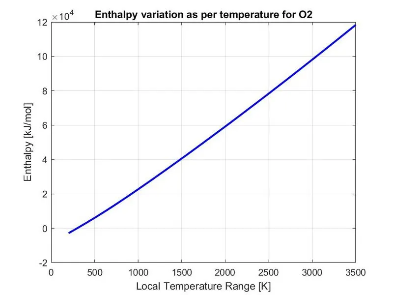
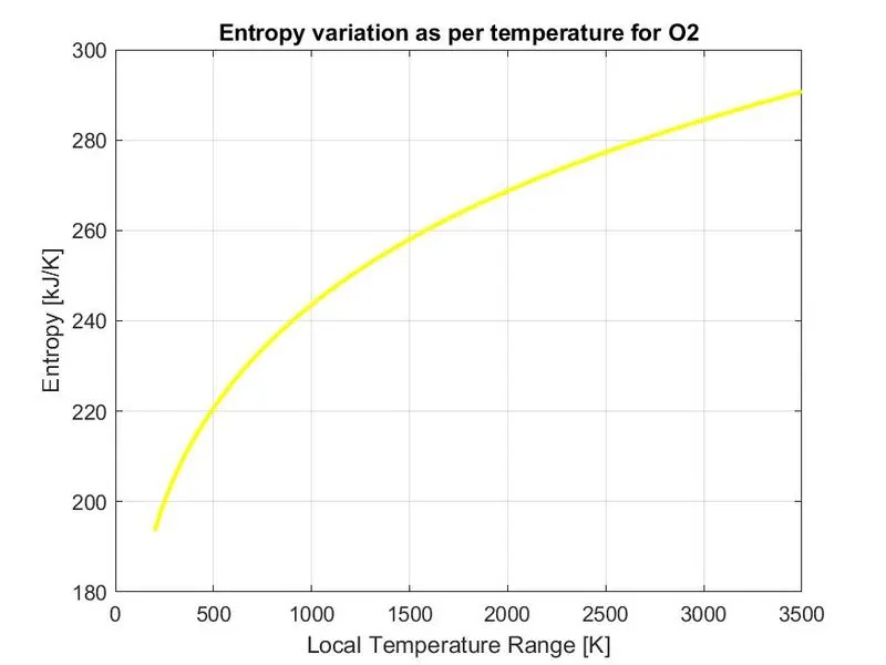
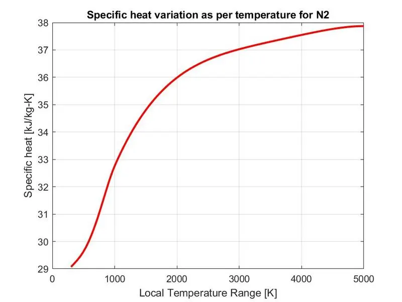
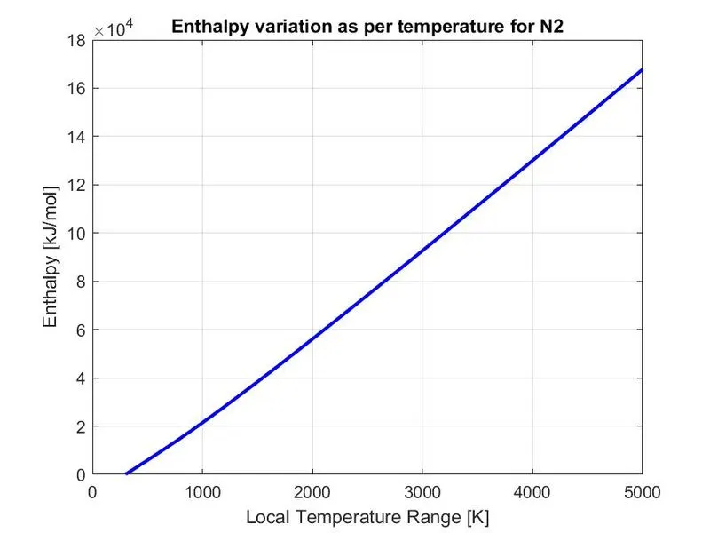
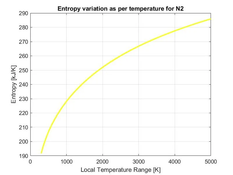
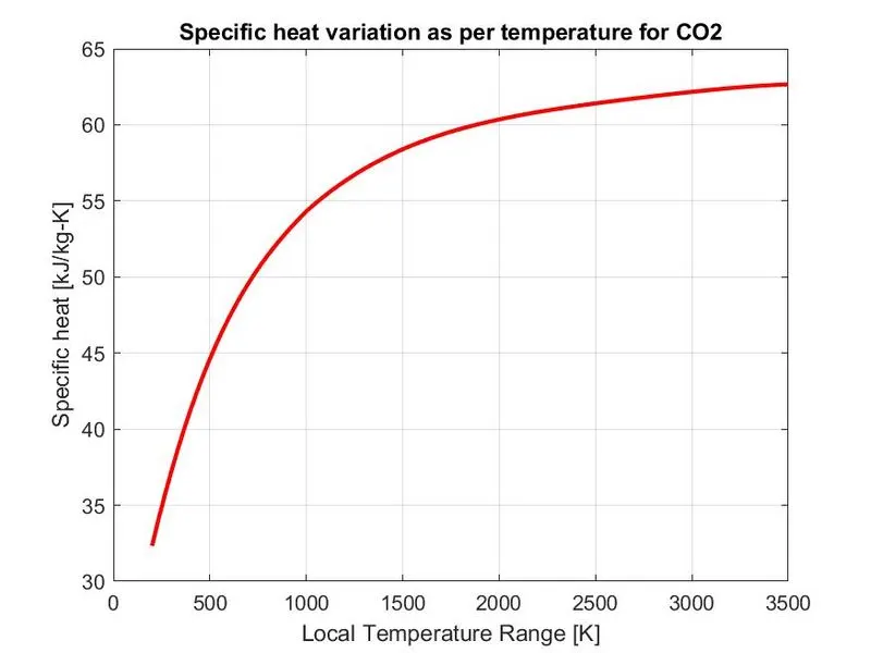
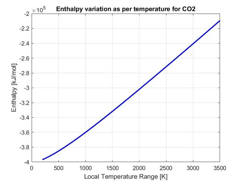
To plot the Cp, Enthalpy and Entropy for the local temperature range (low temperature : high temperature) specific for each species
To save the plots as images with appropriate names and dump them in separate folders for each species with suitable name.

MATLAB code:

Specific heat function

Specific heat in general is the amount of heat required to raise the temperature of a unit mass by 1 degree. This is process dependent. Following code is used to get Cp data.

`(Cp)/T=a_1+a_2*T+a_3*T^2+a_4*T^3+a_5*T^4`

function [Cp]=cp_data(a1,a2,a3,a4,a5,a8,a9,a10,a11,a12,temp,R,global_med_temp)
for i=1:length(temp)
if temp(i) >= global_med_temp
    Cp(i)=R*(a1+(a2*temp(i))+(a3*(temp(i).^2))+(a4*(temp(i).^3))+(a5*(temp(i).^4)));
else
    Cp(i)=R*(a8+(a9*temp(i))+(a10*(temp(i).^2))+(a11*(temp(i).^3))+(a12*(temp(i).^4)));
end
end
end

Here, 'Cp' function requires coefficients shown in Cp polynomial, gas constant, local temperature range and global medium temperature. Global medium temperature and local medium temperature are having same value. As the first seven coefficients are for high temperature and the remaining are for low temperature, one has to compare local temperature values with global medium temperature. So, 'if else' loop is used. Here, 'temp' is an array of local temperatures defined for respective species.

Enthalpy function

Enthalpy is a property of a thermodynamic system, and is defined as the sum of the system's internal energy and the product of its pressure and volume. Following code is used to get enthalpy(H) data.

`H/(RT)=a_1+a_2*(T/2)+a_3*((T^2)/3)+a_4*((T^3)/4)+a_5*((T^4)/5)+a_6/T`

function [H]=h_data(a1,a2,a3,a4,a5,a6,a8,a9,a10,a11,a12,a13,temp,R,global_med_temp)
for i=1:length(temp)
if temp(i) >= global_med_temp
    H(i)=R*temp(i).*(a1+(a2*temp(i).*0.5)+(a3*(temp(i).^2)/3)+(a4*(temp(i).^3)*0.25)+(a5*(temp(i).^4)/5)+(a6./temp(i)));
else
    H(i)=R*temp(i).*(a8+(a9*temp(i).*0.5)+(a10*(temp(i).^2)/3)+(a11*(temp(i).^3)*0.25)+(a12*(temp(i).^4)/5)+(a13./temp(i)));
end
end
end

Above code is same as that for Cp except the polynomial is for enthalpy.

Entropy function

Entropy is the measure of a system's thermal energy per unit temperature that is unavailable for doing useful work. It is also a measure of the molecular disorder, or randomness, of a system. Following code is used to get entropy(S) data.

`S/R=a_1*lnT+a_2*T+a_3*(T^2/2)+a_4*(T^3/3)+a_5*(T^4/4)+a_7`

function [S]=s_data(a1,a2,a3,a4,a5,a7,a8,a9,a10,a11,a12,a14,temp,R,global_med_temp)
for i=1:length(temp)
if temp(i) >= global_med_temp
    S(i)=R*((a1*log(temp(i)))+(a2*temp(i))+(a3*(temp(i).^2)/2)+(a4*(temp(i).^3)/3)+(a5*(temp(i).^4)/4)+a7);
else
    S(i)=R*((a8*log(temp(i)))+(a9*temp(i))+(a10*(temp(i).^2)/2)+(a11*(temp(i).^3)/3)+(a12*(temp(i).^4)/4)+a14);
end
end
end

Above code is same as that for Cp except the polynomial is for entropy.

Molecular weight function

The molecular weight is the weight of a given molecule. It is measured in daltons (Da or u). It is calculated from the standard atomic weights of each elements. Following code is used to get molecular weight data.

#Inputs

function Molecular_weight=MolecularW(Species)
atom_name=['O','H','C','N','S','A'];
atm_w=[16 1 12 14 32 40];

Here, 'Molecular_weight' array saves the molecular weights of different species. The list of species comprises of 'O', 'H', 'C', 'N', 'S', 'A' these elements saved in 'atom_name'. Their atomics weights are stored in 'atm_w'.

#Calculations for molecular weight

for i=1:length(Species)
    for j=1:length(atom_name)
        if strcmpi(Species(i),atom_name(j))
            Molecular_weight=Molecular_weight+atm_w(j);
            m=j;
        end
    end
           
            n=str2num(Species(i));
            if n>1
                Molecular_weight=Molecular_weight+atm_w(m)*(n-1);
            end
end

Initially, 'Molecular_weight' stores '0' value. 'for' loop is used to calculate molecular weight of respective species. Here, we use length parameter of Species, which is used to identify elements in that species. Also, length of atom_name is used for comparison. 'strcmpi' command compare 'Species' with 'atom_name' irrespective of its case (i.e. upper case or lower case). So, for every element which is identified, it's atomic weight is added to the 'Molecular_weight'. For some species, along with elements, there are number of elements. So, one need to add multiple of atomic weights of that element. This is done by storing its position in a variable 'm'. So, cascading of 'for' and 'if-else' loop helps for this. As, 'Species' is a string, one needs to convert the number of element into a numerical value. This is done by using 'str2num' command. 'if-else' loop is used to add that extra number of elemets to the sum of Molecular_weight.

#Data and file saving

MW_f=fopen('MW_data.txt','a+');
fprintf(MW_f,'Molecular weight of %s ',Species);
fprintf(MW_f,'is %d\n',Molecular_weight);
fclose(MW_f);
fprintf('Molecular weight of %s ',Species)
fprintf('is %d\n',Molecular_weight)
end

'fopen' command creates a text file and it's extension 'a+' adds the molecular weight data after each iteration. 'fprintf' writes text in text file. 'fclose' closes the file. The other 'fprintf' command shows text i.e molecular weight of particular species, in command window after each iteration.

Main code

close all
clear all
clc
%Open file 'THERMO.dat' and read it
f1=fopen('THERMO.dat','r');
fgetl(f1);
%Assigning global temperatures
A=fscanf(f1,'%f',[1 3]);
global_low_temp=A(1);
global_med_temp=A(2);
global_high_temp=A(3);

for i=1:4
    fgetl(f1);
end

Here, 'fscanf' command reads data from text file 'THERMO.dat'. Consecutively, global temperature range is stored in variables. 'fgetl' reads line from text.

%Loop for all species data collection
for i=1:53
data=fgetl(f1);
%Splitting data into an array and assigning local max and min for
%respective species
B=strsplit(data,' ');
n=length(B);
Species=(B{1});
local_min_temp=str2num(B{n-3});
local_max_temp=str2num(B{n-2});

Here, 'for' loop is used to run the code for 53 species. 'strsplit' command splits a string into number of strings. From this splitted string, Species name, local minimum and maximm temperatures are collected and saved into variables.

%Extracting coefficients
    C=fgetl(f1);
    a=findstr(C,'E');
    %First 7 coefficients for high temperature(i.e more than local medium)
    a1=C(1:a(1)+3);
    a1=str2num(a1);
    a2=C(a(1)+4:a(2)+3);
    a2=str2num(a2);
    a3=C(a(2)+4:a(3)+3);
    a3=str2num(a3);
    a4=C(a(3)+4:a(4)+3);
    a4=str2num(a4);
    a5=C(a(4)+4:a(5)+3);
    a5=str2num(a5);
    D=fgetl(f1);
    b=findstr(D,'E');
    a6=D(1:b(1)+3);
    a6=str2num(a6);
    a7=D(b(1)+4:b(2)+3);
    a7=str2num(a7);
    %Remaining 7 for low temperature(i.e. less than local medium)
    a8=D(b(2)+4:b(3)+3);
    a8=str2num(a8);
    a9=D(b(3)+4:b(4)+3);
    a9=str2num(a9);
    a10=D(b(4)+4:b(5)+3);
    a10=str2num(a10);
    E=fgetl(f1);
    c=findstr(E,'E');
    a11=E(1:c(1)+3);
    a11=str2num(a11);
    a12=E(c(1)+4:c(2)+3);
    a12=str2num(a12);
    a13=E(c(2)+4:c(3)+3);
    a13=str2num(a13);
    a14=E(c(3)+4:c(4)+3);
    a14=str2num(a14);

In 'THERMO.dat' file, for each species, there are 14 coefficients for the polynomials explained above. Each coefficient has it's numerical value in the form of number and exponential term i.e. E. To find this 'E', 'findstr' command is used. After 'E', there are 3 terms and after that 3 terms, there is a new coefficient. So, with this logic, one can take specific coefficient from the list of coefficients. The above code, is for the specific species. Like this, one can evaluate coefficients for other species.

%Gas constant
R=8.314;
temp=linspace(local_min_temp,local_max_temp,100);
%Molecular weights calculations and its saving in a folder 
Molecular_weight(i)=MolecularW(Species);

'temp' is an array which saves number of temperature values within local minimum and local maximum with respect to the species. 'MolecularW(Species)' calls the function for molecular weight calculation.

%Creating a folder for storing species data
c_d=pwd;
mkdir(Species);
cd(Species);

'pwd' identifies current directory and it's location is saved in 'c_d'. 'mkdir' creates a new directory with a name of species and cd(Species) makes a newly created directory as current directory.

%Plotting Cp/H/S Vs. temp for all species
%Cp data
figure(1)
[Cp]=cp_data(a1,a2,a3,a4,a5,a8,a9,a10,a11,a12,temp,R,global_med_temp);
plot(temp,Cp,'linewidth',2,'color','r')
xlabel('Local Temperature Range [K]')
ylabel('Specific heat [kJ/kmol-K]')
title(sprintf('Specific heat variation as per temperature for %s',Species))
grid on
saveas(figure(1),'Specific heat Vs. Temperature.jpg')
%H data
figure(2)
[H]=h_data(a1,a2,a3,a4,a5,a6,a8,a9,a10,a11,a12,a13,temp,R,global_med_temp);
plot(temp,H,'linewidth',2,'color','b')
xlabel('Local Temperature Range [K]')
ylabel('Enthalpy [kJ/mol]')
title(sprintf('Enthalpy variation as per temperature for %s',Species))
grid on
saveas(figure(2),'Enthalpy Vs. Temperature.jpg')
%S data
figure(3)
[S]=s_data(a1,a2,a3,a4,a5,a7,a8,a9,a10,a11,a12,a14,temp,R,global_med_temp);
plot(temp,S,'linewidth',2,'color','y')
xlabel('Local Temperature Range [K]')
ylabel('Entropy [kJ/K]')
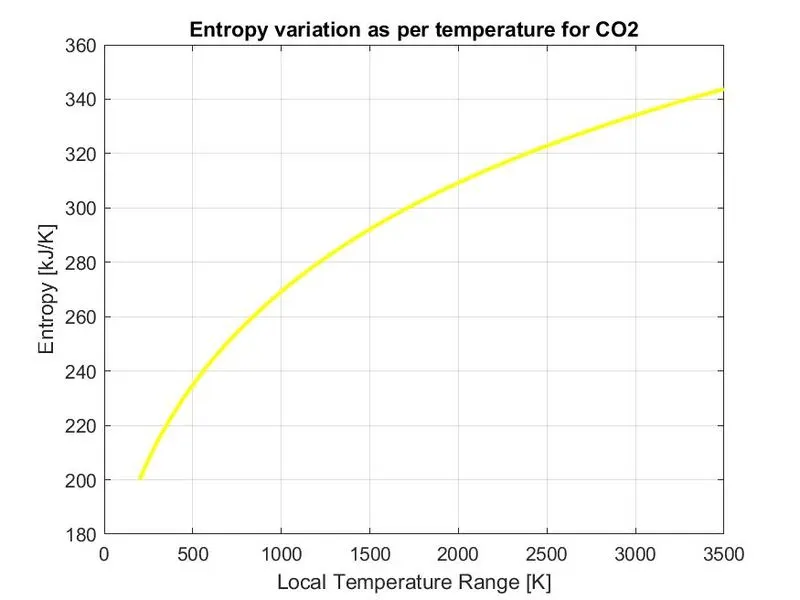
title(sprintf('Entropy variation as per temperature for %s',Species))
grid on
saveas(figure(3),'Entropy Vs. Temperature.jpg')
cd(c_d);
end

All data of Cp, H and S are saved in respective species directory. 'saveas' command saves the plots as image files in respective species directory. Cp, H and S functions are called using respective function's name. Consecutively, their plots are created using 'plot' command, labels and titles are given. The above code runs for each species, so to save new data in new species folder, 'cd(c_d)' command is used.

MATLAB Output:

Screenshot of the window where all the folders are saved

Plots of O2

#Cp Vs. Temperature range

#H Vs. Temperature range

#S Vs. Temperature range

Plots of N2

#Cp Vs. Temperature range

#H Vs. Temperature range

#S Vs. Temperature range

Plots of CO2

#Cp Vs. Temperature range

#H Vs. Temperature range

#S Vs. Temperature range

Output of Molecular weights

Conclusion:

While writing a program for data parsing, one should be aware of the arrangement of data in text file. After getting the data in required format, it is quite easy to manipulate.

References:

Project 1 - Parsing NASA thermodynamic data

Ship work like this
in your own course.

Talk to a career counsellor

Ship work like thisin your own course.

Talk to a career counsellor

Ship work like this
in your own course.