Project 2 - Rankine cycle Simulator

Aim:

To create a Rankine Cycle Simulator using MATLAB

Theory:

Rankine cycle is the theoretical cycle on which the steam turbine (or engine) works.

The schematic diagram and T-s diagram of Rankine Cycle, are given as follows,

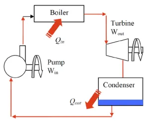
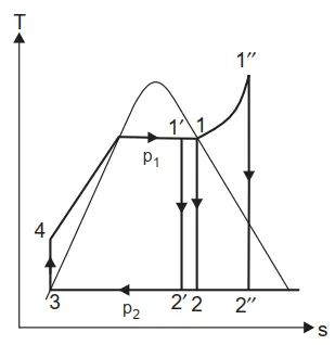
It comprises of the following processes :

Process 1"-2" : Reversible adiabatic expansion in the turbine (or steam engine). The superheated vapor expands through a turbine, generating power. This decreases the temperature and pressure of the vapor, and some condensation may occur.

Process 2"-3 : Constant-pressure transfer of heat in the condenser. The slightly wet vapor at 2 then enters a condenser where it is condensed at a constant pressure to become a saturated liquid-vapor mixture, and finally a saturated liquid (at 3). Heat Qout is given off as a result of the enthalpy of vaporization resulting from condensation of the vapor.

Process 3-4 : Reversible adiabatic pumping process in the feed pump. The working fluid is pumped from low to high pressure (at 4). Because the fluid is a liquid at this stage (it lies to the left of the saturated liquid line in the compressed liquid region), the pump requires relatively little input energy.

Process 4-1" : Constant-pressure transfer of heat in the boiler. The high pressure compressed liquid enters a boiler where it is heated at constant pressure by an external heat source to become first a saturated liquid, then a saturated liquid-vapor mixture, then a superheated vapor (ending at 1", a subcritical state having T1" < Tcr).

Net work(`W_(nt)`)

The net work is the difference between turbine work (`W_(turb)`) and pump work (`W_(pump)`) i.e.

`W_(nt)=W_(turb)-W_(pump)`

Efficiency of Rankine cycle(`eta`)

`eta=(W_(nt)/Q_(s))*100`

where, `Q_(s)` is heat supplied by boiler.

Back work ratio(BWR)

`BWR=W_(pump)/W_(turb)`

Objectives:

• To calculate the state points of the Rankine Cycle based on user inputs.
• To plot the corresponding T-s and h-s plots for the given set of inputs.

MATLAB Code:

clear all
close all
clc

fprintf('1-2: Reversible adiabatic expansion\n')
fprintf('1-2: Constant pressure heat rejection\n')
fprintf('1-2: Reversible adiabatic compression\n')
fprintf('1-2: Constant pressure heat addition\n\n')

'fprintf' shows the content described in command itself. Here, description about processes is there.

%inputs
%Turbine inlet temp
t1=input('Enter turbine inlet temperature(in Degree Celcius):');
%Turbine inlet pressure
p1=input('Enter turbine inlet pressure(in bar):');
%Condenser inlet pressure
p2=input('Enter condenser inlet pressure(in bar):');

Here, inputs such as turbine inlet temperature, turbine inlet pressure, condenser inlet pressure, are taken from user. For that, 'input' command is used.

%State 1
h1=XSteam('h_pT',p1,t1);
s1=XSteam('s_pT',p1,t1);

'XSteam' is a program for steam table. Here, values of enthalpy at state 1 i.e. h1 and entropy at state 1 i.e. s1 are derived from 'XSteam.m' file. 'h_pt' requires pressure and temperature values to get enthalpy value. Same logic applies to s1.

%State 2
sf_p2=XSteam('sL_p',p2);
sg_p2=XSteam('sV_p',p2);
sfg_p2=sg_p2-sf_p2;
s2=s1;

Saturated vapor and saturated liquid entropy values at state 2 are calculated based on condenser pressure. As, process 1-2 is an isentropic process, entropy remains same.

%dryness fraction
x2=(s1-sf_p2)/sfg_p2;
hf_p2=XSteam('hL_p',p2);
hg_p2=XSteam('hV_p',p2);
hfg_p2=hg_p2-hf_p2;
h2=hf_p2+(x2*hfg_p2);
vf_p2=XSteam('vL_p',p2);
t2=XSteam('T_hs',h2,s2);

To calculate the enthalpy at state 2, we need to find value of dryness fraction. The formula for this is given in code itself. Consecutively, tempearture at state 2 i.e. t2 is calculated. The value of saturated vapor specific volume i.e. vf at p2, is required to calculate pump work.

%State 3
h3=hf_p2;
t3=t2;
s3=XSteam('s_ph',p2,h3);
p3=p2;

As at state 3, the working fluid is in liquid form, its enthalpy will be same as that of saturated vapor enthalpy at pressure,p2. For process 2-3, tempearture and pressure remain same.

%Work done on pump
w_P=vf_p2*(p1-p2)*10^2;

The value of vf at p2, calculated earlier, is used here to calculate pump work.

%State 4
h4=w_P+h3;
s4=s3;
p4=p1;
cp4=XSteam('Cp_ps',p4,s4);
cv4=XSteam('Cv_ps',p4,s4);
y=cp4/cv4;
t4=t3*((p4/p3)^((y-1)/y));

Process 3-4 is an isentropic process, so the entropy remains constant. Specific heat at constant pressure i.e. Cp and specific heat at constant volume i.e. Cv, at state 4, are calculated with the help of 'XSteam.m' file. Gamma, 'y' is a specific heat ratio, required to calculate tempearture at state 4 i.e. t4 with the help of `pv^gamma=c`.

%Work done by turbine
w_T=h1-h2;
%Net work
w_net=w_T-w_P;
%Heat supplied
q_s=h1-h4;
%Efficiency
eta=(w_net/q_s)*100;
%Back work ratio
bwr=w_P/w_T
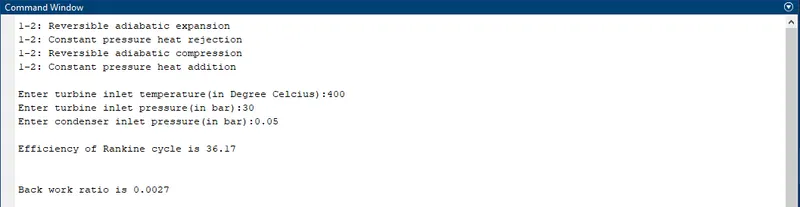
fprintf('\nEfficiency of Rankine cycle is %2.2f\n\n',eta)
fprintf('\nBack work ratio is %2.4f\n\n',bwr)

Here, with all state properties, one can calculate work done by turbine, net work, heat supplied, efficiency and back work ratio.

t4_1=XSteam('Tsat_p',p1);
sf4_1=XSteam('sL_T',t4_1);
sg4_1=XSteam('sV_P',p1);

These are values of temperature, saturated vapor and saturated liquid entropy at points where constant pressure line at pressure p1, intersects saturation line. These points lie between process 4-1.

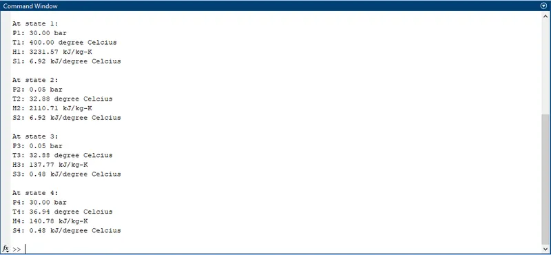
fprintf('At state 1:\nP1: %3.2f bar\nT1: %3.2f degree Celcius\nH1: %4.2f kJ/kg-K\nS1: %3.2f kJ/degree Celcius\n\n',p1,t1,h1,s1)
fprintf('At state 2:\nP2: %3.2f bar\nT2: %3.2f degree Celcius\nH2: %4.2f kJ/kg-K\nS2: %3.2f kJ/degree Celcius\n\n',p2,t2,h2,s2)
fprintf('At state 3:\nP3: %3.2f bar\nT3: %3.2f degree Celcius\nH3: %4.2f kJ/kg-K\nS3: %3.2f kJ/degree Celcius\n\n',p3,t3,h3,s3)
fprintf('At state 4:\nP4: %3.2f bar\nT4: %3.2f degree Celcius\nH4: %4.2f kJ/kg-K\nS4: %3.2f kJ/degree Celcius\n\n',p4,t4,h4,s4)

These show values of pressure, tempearture, enthalpy and entropy at state 1, 2, 3, 4 respectively.

%Liquid-Vapour line
temp=linspace(1,370,50);
for i=1:length(temp)
    S_L(i)=XSteam('sL_T',temp(i));
    S_V(i)=XSteam('sV_T',temp(i));
    H_L(i)=XSteam('hL_T',temp(i));
    H_V(i)=XSteam('hV_T',temp(i));
end

Here, 'for' loop is used to generate saturation line in T-s plot. To plot the saturation line, one needs to take a temperature range (i.e. 'linspace' command) and using these values in 'XSteam' function, one can get values of saturated vapor entropy/enthalpy and saturated liquid entropy/enthalpy.

%Plotting T-s diagram
subplot(1,2,1)
plot([s1 s2 s3 s4 sf4_1 sg4_1 s1],[t1 t2 t3 t4 t4_1 t4_1 t1],'color','k','marker','o','markerfacecolor','b')
hold on
plot(S_L,temp,'color','r')
plot(S_V,temp,'color','r')
axis([0 10 0 450])
text(s1,t1,' 1')
text(s2,t2,'  2')
text(s3,t3,'  3')
text(s4,t4,'  4','HorizontalAlignment','right')
xlabel('Entropy [kJ/degree C]')
ylabel('Temperature [Celcius]')
title('T-s Diagram')
legend('Process line','Saturation line','location','northwest')

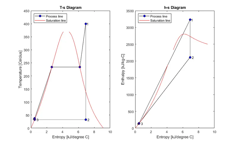
'subplot' command let you accomodate number of plots in a single window. Here, T-s diagram and h-s diagram are two plots. In T-s plot, all the state points are joined, with 'plot' command. 'axis' command lets you fix an axis. 'text' command lets you write text for points on plot. Labels, titles, legends are given with commands shown in the above code.

%Plotting h-s diagram
subplot(1,2,2)
plot([s1 s2 s3 s4 s1],[h1 h2 h3 h4 h1],'color','k','marker','o','markerfacecolor','b')
hold on
plot(S_L,H_L,'color','r')
plot(S_V,H_V,'color','r')
text(s1,h1,' 1')
text(s2,h2,'  2')
text(s3,h3,'  3')
text(s4,h4,'  4','HorizontalAlignment','right')
xlabel('Entropy [kJ/degree C]')
ylabel('Enthalpy [kJ/kg-C]')
title('h-s Diagram')
legend('Process line','Saturation line','location','northwest')

Similarly, for plotting h-s diagram, above commands are used. The descriptions for above code is same as that for T-s diagram.

MATLAB Output:

Efficiency of Rankine cycle, Back work ratio

T-s diagram and h-s diagram plots

Conclusion:

This code takes turbine inlet tempearture, turbine inlet pressure, condenser inlet pressure as user-inputs and gives state properties, efficiency and T-s, h-s diagrams as outputs.

References:

• https://www.mcgoodwin.net/pages/thermodynamics.pdf
• https://www.sciencedirect.com/topics/engineering/back-work-ratio
• Book of Engineering Thermodynamics by R. K. Rajput.