Week 7 - Simulation of a 1D Super-sonic nozzle flow simulation using Macormack Method
AIM- To perform the simmulation of a 1D super sonic nozzel using MacCormack's method.
THEORY- A supersonic nozzel is a convergent and divergent type of nozzel, consisting of a converging part at the first end and the divergent part at the other along with a norrow throat section between the two parts.The pressure, temperature ,density,velocity and area in different parts of the nozzel are assumed to be p0,T0,`rho0`,v0 respectively at the convergent section and area in this section is assumed to be infinity since the convergent section is connected to the reservoir.Similarly at the exit pe,Te,`rhoe`,ve are the respective parameters.
In a supersonic nozzel a pressure fluid enters the nozzel from the convergent section and exits from the divergent section at supersonic speed.
The mach number is a dimensionless number whic determines the speed of the fluid at different cross sections
M=u/c
where, u = local vlocity of flow in m/s.
c=speed of sound.
At the convergent section mach number is less than 1 i.e the local velocity if flow is less than the speed of sound where as at the divergent section the mach number is greater than 1 determining the velocity of flow is greater than the speed of sound, at the throat section the mach number is equal to 1 i.e velocity of flow and speed of sound are equal.
In this project we will perform the simulations for both conservative and non conservative form of the Navier Stokes equations and compare the results.
#Non conservative form-
1.The continuity,momentum and energy equations for the non conservative form of a 1D supersonic nozzel are as follows.
Continuity equation-
`(delrho)/(delt)=-rho.(delv)/(delx)-(rho.v.(dellog(a))/(delx))-v.(delrho/delx)`
2.Momentum equation-
`(delv)/(delt)=-v.(delv)/(delt)-(1/gamma.((delT)/(delx)+(T/rho.(delrho)/(delx))))`
3.Energy equation-
`(delT)/(delt)=-v.(delT)/(delx)-((gamma-1).T.((delv)/(delx)+(v.(dellog(a))/(delx))))`
The equations above are solved using Maccormack's method as follows.
1.Defining the initial conditions.
2.Applying the predictor method to all the three equations by forward differencing.
a.Continuity equation-
`(delrho)/(delt)=-rho(i).((v(i+1)-v(i))/(delx))-(rho(i).v(i).``((loga(i+1)-loga(i))/(delx)))``-v(i).((rho(i+1)-rho(i))/(delx))`
b.Momentum equation-
`(delv)/(delt)=-v(i).((v(i+1)-v(i))/(delx))-(1/gamma.((T(i+1)-T(i))/(delx))``((T(i))/(rho(i)).((rho(i+1)-rho(i))/(delx)))`
c.Energy equation-
`(delT)/(delt)=-v(i).((T(i+1)-T(i))/(delx))``((gamma-1).T(i)(((v(i+1)-v(i))/(delx))+``(v(i).((loga(i+1)-loga(i))/(delx))))`
3.After the predictor step all the values are updated to at all the grid points.
4.Then the corrector step is applied in which the euations on the right hand side are backward differenced.
a.Continuity equation-
`(delrho)/(delt)=-rho(i).((v(i)-v(i-1))/(delx))``-(rho(i).v(i).((loga(i)-loga(i-1))/(delx)))``-v(i).((rho(i)-rho(i-1))/(delx))`
b.Momentum equation-
`(delv)/(delt)=-v(i).((v(i)-v(i-1))/(delx))``-(1/gamma.((T(i)-T(i-1))/(delx))+((T(i))/(rho(i)).((rho(i)-rho(i-1))/(delx)))`
c.Energy equation-
`(delT)/(delt)=-v(i).((T(i)-T(i-1))/(delx))-``((gamma-1).T(i).(((v(i)-v(i-1))/(delx))+((v(i).((loga(i)-loga(i-1))/(delx))))`
5.Computing the average, the average for conituity,momentum and energy equations are calculated by multiplying the sum of partial differential equations of predictor and corrector step by 0.5.
6.Then the final update is done by using the average value computed above.
7.The boundary conditions at each step are updated as follows.
Inlet- v(1)=2*v(2)-v(3)
Outlet- v(n)=2*v(n-1)-v(n-2)
rho(n)=2*rho(n-1)-rho(n-2)
T(n)=2*T(n-1)-T(n-2)
#Conservative form-
In conservative form the equations are not expressd in terms of primitive variables but in terms of solution terms(U) ,flux terms(F) ,source terms(J).
a.Continuity equation-
`(del(rho.a))/(delt)+(del(rho.a.v))/(delx)=0`
b.Momentum equation-
`(del(rho.a.v))/(delt)+((del(rho.a.v^2+(1/gamma).p.a))/(delt))=``p.(1/gamma).(dela)/(delx)`
c.Energy equation-
`(del((rho.a.(e/gamma-1))+((gamma/2).v^2)))/(delt)+``(del(rho.a.v.(e/(gamma-1)+(gamma/2).v^2))+p.a.v)/(delx)=0`
To express the equations in terms of solution vectors,flux vectors and source term
Solution vectors are defined as follows-
U1=`rho.a`
U2=`rho.a.v`
U3=U1.`((T/(gamma-1))+(gamma/2).v^2)`
Flux terms are as follows-
F1=U2
F2=`((U2)^2/(U1)+((gamma-1)/gamma.(U3-(gamma.0.5.(U2)^2)/(U1))))`
F3=`(gamma.U3.U2)/(U1)-((gamma.0.5.(gamma-1).(U2)^3)/(U1)^2)`
Source term is as follows-
J2=`(1/gamma).rho.T.(dela)/(delx)`
Now, the governing equations can be expressed as follows.
Continuity equation-
`(delU1)/(delt)=-(delF1)/(delx)`
Momentum equation-
`(delU2)/(delt)=-(delF2)/(delx)+J2`
Energy equation-
`(delU3)/(delt)=-(delF3)/(delx)`
Now, these euations are used in MacCormack's method.
1.Setting up of initial conditions
The initial conditions for conservative form are different from those of non conservative form.
for 0<=x<=0.5, rho=1, T=1
for 0.5<=x<=1.5,
rho=1-0.366*(x-0.5)
T=1-0.167*(x-0.5)
for 1.5<=x<=3.5
rho=0.634-0.3897*(x-1.5)
T=0.83-0.3507*(x-1.5)
2.Predictor method
Continuity equation-
`(delU1)/(delt)=-((F1(i+1)-F1(i))/(delx))`
Momentum equation-
`(delU2)/(delt)=-((F2(i+1)-F2(i))/(delx))+J2`
Energy equation-
`(delU3)/(delt)=-((F3(i+1)-F3(i))/(delx))`
3.The values of all the solution vectors are then updated at all grid points.
4.The corrector step is then applied as follows.
Continuity equation-
`(delU1)/(delt)=-((F1(i)-F1(i-1))/(delx))`
Momentum equation-
`(delU2)/(delt)=-((F2(i)-F2(i-1))/(delx))+J2`
Energy equation-
`(delU3)/(delt)=-((F3(i)-F3(i-1))/(delx))`
5.Computing the average, the average for conituity,momentum and energy equations are calculated by multiplying the sum of partial differential equations of predictor and corrector step by 0.5.
6.Final update is performed as follows,
U1(i)=U1_old(i)+(`((delU1)/(delt))avg``(i).delt)`
U2(i)=U2_old(i)+`(((delU2)/(delt))avg(i).delt)`
U3(i)=U3_old(i)+`(((delU3)/(delt))avg(i).delt)`
7.The boundary conditions at each step are updated as follows.
U1(1)=2*U1(n-1)-U1(n-2)
U2(1)=2*U2(n-1)-U2(n-2)
U3(1)=2*U3(n-1)-U3(n-2)
`rho=(U1)/a`
`v=(U2)/(U1)`
`T=(gamma-1).((U3)/(U1)-(gamma/2).v^2)`
MAIN CODE-
close all
clear all
clc

n=31;
x=linspace(0,3,n);
dx=x(2)-x(1);
L=3;                %length of the nozzel
nt=1400;            %number of time steps
CFL = 0.5;          % Courant Number
a = 1 + 2.2*(x-1.5).^2;

tic
[rho_nc,T_nc,v_nc,p_nc,mach_nc,rho_tr_nc,p_tr_nc,T_tr_nc,mach_tr_nc,mass_flow_nc,mass_flow_tr_nc]=nonconserv_n(x,n,nt,dx,a);
time_nc = toc;

[rho_c,T_c,v_c,p_c,mach_c,rho_tr_c,T_tr_c,p_tr_c,mach_tr_c,mass_flow_c,mass_flow_tr_c]=consrv_n(x,n,nt,dx,a);
time_c=toc;

%Steady state variation of primitive variables
figure(1)
subplot(4,1,1)
plot(x,rho_c,'b','linewidth',2)
hold on
plot(x,rho_nc,'*r')
ylabel('Density')
xlabel('Nozzle length')
title('Steady state variation of primitive variables')
subplot(4,1,2)
plot(x,T_c,'b','linewidth',2)
hold on
plot(x,T_nc,'*r')
ylabel('Temperature')
xlabel('Nozzle length')
subplot(4,1,3)
plot(x,p_c,'b','linewidth',2)
hold on
plot(x,p_nc,'*r')
ylabel('Pressure')
xlabel('Nozzle length')
subplot(4,1,4)
plot(x,mach_c,'b','linewidth',2)
hold on
plot(x,mach_nc,'*r')
ylabel('Mach number')
xlabel('Nozzle length')

%Transient variation of primitive variables at throat
figure(2)
subplot(4,1,1)
plot(rho_tr_c,'b')
hold on
plot(rho_tr_nc,'r')
ylabel('Density')
xlabel('Timestep')
title('Transient variation of primitive variables')
legend('conservative','Non-conservative')
subplot(4,1,2)
plot(T_tr_c,'b')
hold on
plot(T_tr_nc,'r')
ylabel('Temperature')
xlabel('Timestep')
subplot(4,1,3)
plot(p_tr_c,'b')
hold on
plot(p_tr_nc,'r')
ylabel('Pressure')
xlabel('Timestep')
subplot(4,1,4)
plot(mach_tr_c,'b')
hold on
plot(mach_tr_nc,'r')
ylabel('Mach number')
xlabel('Timestep')

%Steady state variation of Mass flow rate
figure(3)
plot(x,mass_flow_c,'b')
hold on
plot(x,mass_flow_nc,'r')
title('Steady state variation of Mass flow rate')
legend('Conservative','Non-conservative')
FUNCTION CODE FOR NON-CONSERVATIVE FORM-
function [rho,T,v,p,mach,rho_tr,p_tr,T_tr,mach_tr,mass_flow,mass_flow_tr]=nonconserv_n(x,n,nt,dx,a);

  %defining the initial conditions

  rho=1-(0.3146.*x);
  T=1-(0.2314.*x);
  v=(0.1+(1.09.*x)).*(T.^0.5);
  gamma=1.4;


  %defining dt
  %dt = min(CFL*dx./(v+sqrt(T))); % Explicit CFL = [|u|+|a|]*dt/dx; min function returns a single value
  dt = 0.0201;


  %copy of initial values
  rho_old=rho;
  T_old=T;
  v_old=v;


%simplifying the Maccormack's method 1d nozzel flow equation by to avoide errors due to length of equation.
%continuity equation
%drho/dt=-rho*(dv/dx)-(rho*v*d(loga)/dx)-v*(drho/dx)

%momentum equation
%dv/dt=-v*(dv/dt)-(1/gamma)*(dt/dx+((T/rho)*drho/dx)

%energy equation
%dT/dt=-v*(dT/dx)-(gamma-1)*T*((dv/dx)+v*d(loga)/dx)

for k=1:nt;
  rho_old=rho;
  T_old=T;
  v_old=v;

  for i=2:n-1;
    %predictor step
    dvdx=(v(i+1)-v(i))/dx;
    drhodx=(rho(i+1)-rho(i))/dx;
    dTdx=(T(i+1)-T(i))/dx;
    dadx=(log(a(i+1))-log(a(i)))/dx;

    %continuity equation
    drhodt_p(i)=(-1*rho(i)*dvdx)-(rho(i)*v(i)*dadx)-(v(i)*drhodx);

    %momentum equation
    dvdt_p(i)=(-v(i)*dvdx)-((1/gamma)*((dTdx)+((T(i)/rho(i)*drhodx))));

    %energy equation
    dTdt_p(i)=(-v(i)*dTdx)-((gamma-1)*T(i)*(dvdx+v(i)*dadx));

  end

  %solution update %% Should be done after predictor loop
  for i=2:n-1;
  rho(i) = rho(i)+(drhodt_p(i)*dt);
  v(i) = v(i)+(dvdt_p(i)*dt);
  T(i) =  T(i)+(dTdt_p(i)*dt);
  end

  %corrector step
  for i=2:n-1;

     %corrector step
    dvdx=(v(i)-v(i-1))/dx;
    drhodx=(rho(i)-rho(i-1))/dx;
    dTdx=(T(i)-T(i-1))/dx;
    dadx=(log(a(i))-log(a(i-1)))/dx;

        %continuity equation
    drhodt_c(i)=(-1*rho(i)*dvdx)-(rho(i)*v(i)*dadx)-(v(i)*drhodx);

    %momentum equation
    dvdt_c(i)=(-v(i)*dvdx)-((1/gamma)*((dTdx)+((T(i)/rho(i)*drhodx))));

    %energy equation
    dTdt_c(i)=(-v(i)*dTdx)-((gamma-1)*T(i)*(dvdx+v(i)*dadx));

  end  %% Loop for corrector should end here

    %finding average
    for m=2:n-1;

      drhodt(m)=0.5*(drhodt_p(m)+drhodt_c(m));
      dvdt(m)=0.5*(dvdt_p(m)+dvdt_c(m));
      dTdt(m)=0.5*(dTdt_p(m)+dTdt_c(m));

    end
  %solution update
  for j=2:n-1
    rho(j)=rho_old(j)+(drhodt(j)*dt);
    v(j)=v_old(j)+(dvdt(j)*dt);
    T(j)=T_old(j)+(dTdt(j)*dt);
  end
  %boundary conditions
  %at inlet
  v(1)=2*v(2)-v(3);

  %At outlet
  v(n) = 2*v(n-1)-v(n-2);
  rho(n) = 2*rho(n-1)-rho(n-2);
  T(n) = 2*T(n-1)-T(n-2);

  p = rho.*T;
  mass_flow = rho.*a.*v;
  mach = v./sqrt(T);

  rho_tr(k) = rho(16);  % rho(16) captures throat value at each timestep
  p_tr(k) = p(16);
  T_tr(k) = T(16);
  mach_tr(k) = mach(16);
  mass_flow_tr(k) = mass_flow(16);

    %Transient state Massflow rate
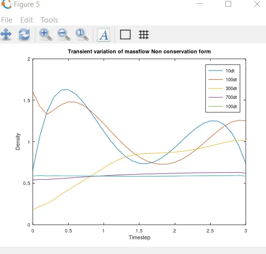
  figure(5)
  if k ==1
    plot(x,mass_flow)
    ylabel('Density')
    xlabel('Timestep')
    title('Transient variation of massflow Non conservation form')
    hold on
  endif
  if k ==10
    plot(x,mass_flow)
  endif
  if k ==100
    plot(x,mass_flow)
  endif
  if k ==300
    plot(x,mass_flow)
  endif
  if k ==700
    plot(x,mass_flow)
  endif
  if k ==1000
    plot(x,mass_flow)
  endif

  end
  legend('10dt','100dt','300dt','700dt','100dt')

endfunction
FUNCTION CODE FOR CONSERVATIVE FORM-
function [rho,T,v,p,mach,rho_tr,T_tr,p_tr,mach_tr,mass_flow,mass_flow_tr]=consrv_n(x,n,nt,dx,a);

  for i=1:n
  %Initial conditions
  if x(i) <= 0.5
    rho(i) = 1;
    T(i) = 1;
  endif

   if x(i) > 0.5 && x(i) <= 1.5
    rho(i) = 1-0.366*(x(i)-0.5);
    T(i) = 1-0.167*(x(i)-0.5);
  endif

    if x(i) > 1.5
    rho(i) = 0.634-0.3897*(x(i)-1.5);
    T(i) = 0.833-0.3507*(x(i)-1.5);
  endif
  end


  gamma=1.4;
  %Definig solution vectors
  U1=rho.*a;
  U2=0.59*ones(1,n);
  v = U2./(rho.*a);
  U3=U1.*((T/(gamma-1))+((gamma/2).*v.^2));

  dt = 0.0267;

  %Application of MacCormack's methods
  for k=1:nt;
    U1_old=U1;
    U2_old=U2;
    U3_old=U3;


    F1=U2;
    F2=((U2.^2./U1)+(((gamma-1)/gamma)*(U3-(gamma.*0.5.*U2.^2)./U1)));
    F3=(((gamma*U3.*U2)./U1)-((gamma*0.5*(gamma-1)*U2.^3)./U1.^2));

    %Predictor step
    for i=2:n-1;
      J2=(1/gamma)*rho(i)*T(i)*((a(i+1)-a(i))/dx);
      %Governing equations
      %dU1/dt=-dF1/dx      ,continuity equation
      %dU2/dt=-dF2/dx +J2  ,momentum equation
      %dU3/dt=-dF3/dx      ,energy equation

      dU1dt_p(i)=-((F1(i+1)-F1(i))/dx);
      dU2dt_p(i)=-((F2(i+1)-F2(i))/dx)+J2;
      dU3dt_p(i)=-((F3(i+1)-F3(i))/dx);

      %solution update
      U1(i)=U1_old(i)+(dU1dt_p(i)*dt);
      U2(i)=U2_old(i)+(dU2dt_p(i)*dt);
      U3(i)=U3_old(i)+(dU3dt_p(i)*dt);


    endfor


    % Predictor update
    F1=U2;
    F2=((U2.^2./U1)+(((gamma-1)/gamma)*(U3-(gamma.*0.5.*U2.^2)./U1)));
    F3=(((gamma*U3.*U2)./U1)-((gamma*0.5*(gamma-1)*U2.^3)./U1.^2));


    rho = U1./a;
    v = U2./U1;
    T = (gamma-1)*(U3./U1 - (gamma*0.5)*v.^2);


    %corrector step
    for j=2:n-1;
      J2=(1/gamma).*rho(j).*T(j).*((a(j)-a(j-1))/dx);

      dU1dt_c(j) = -((F1(j)-F1(j-1))/dx);
      dU2dt_c(j) = -((F2(j)-F2(j-1))/dx)+J2;
      dU3dt_c(j) = -((F3(j)-F3(j-1))/dx);

    endfor

    %computing average
    for m=2:n-1
      dU1dt_avg(m)=0.5*(dU1dt_p(m)+dU1dt_c(m));
      dU2dt_avg(m)=0.5*(dU2dt_p(m)+dU2dt_c(m));
      dU3dt_avg(m)=0.5*(dU3dt_p(m)+dU3dt_c(m));

    endfor

    %final update
    for i=2:n-1;
    U1(i)=U1_old(i)+(dU1dt_avg(i)*dt);
    U2(i)=U2_old(i)+(dU2dt_avg(i)*dt);
    U3(i)=U3_old(i)+(dU3dt_avg(i)*dt);
  end

  rho = U1./a;
  v = U2./U1;
  T = (gamma-1)*(U3./U1 - (gamma*0.5)*v.^2);

  %Boundary conditions
  % At inlet
  U1(1)= rho(1)*a(1);
  U2(1)= 2*U2(2)-U2(3);
  U3(1)= U1(1)*((T(1)/(gamma-1))+(0.5*gamma*(v(1)^2)));

  %At outlet
  U1(n)=2*U1(n-1)-U1(n-2);
  U2(n)=2*U2(n-1)-U2(n-2);
  U3(n)=2*U3(n-1)-U3(n-2);


  p = rho.*T;
  mass_flow = rho.*a.*v;
  mach = v./sqrt(T);

  rho_tr(k) = rho(16);  % rho(16) captures throat value at each timestep
  p_tr(k) = p(16);
  T_tr(k) = T(16);
  mach_tr(k) = mach(16);
  mass_flow_tr(k) = mass_flow(16);

  %Transient state Massflow rate
  figure(4)
 if k ==1
    plot(x,mass_flow)
    ylabel('Density')
    xlabel('Timestep')
    title('Transient variation of massflow Conservation form')
    hold on
 endif
 if k ==10
    plot(x,mass_flow)
 endif
 if k ==100
    plot(x,mass_flow)
 endif
 if k ==300
    plot(x,mass_flow)
 endif
 if k ==700
    plot(x,mass_flow)
 endif
 if k ==1000
    plot(x,mass_flow)
  endif

 end
 legend('10dt','100dt','300dt','700dt','100dt')

endfunction
RESULTS-
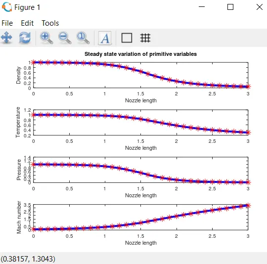
1. From the variation of primitive variables along the nozzel length it can be ifered that density, temperature and pressure tends to drop gradually where as the mach number rises across the nozzel length for non-conservative(red*) and conservative(blue) forms.
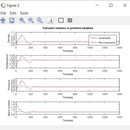
2.Time wise variation of primitive variables shows unstability of primitive variables in non coonservative form initially with the increasing timesteps both the forms exhibit stable trends with non conservative form being more efficient as compared to conservative form.
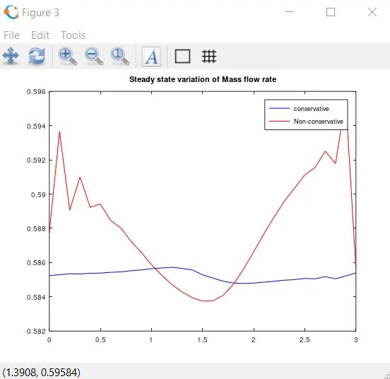
3.Variation of mass flow rate across the nozzel length is found more in non-conservative form which is found to be highly unstable where as the conservative form shows a stable trend.
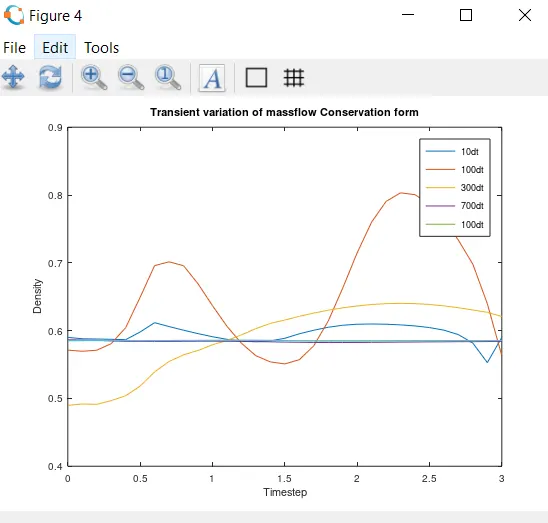
4.The transient variation of massflow for conservation form shows unstability at lower time steps and becomes stable at higher time steps.
5.Similar to conservation form ,the non conservative form also exhibits unstability at the initial time steps but shows comparitively more fluctuation, however, it becomes stable at higher timesteps just like the non conservative form.
CONCULISION-
1.Non conservative form will be best suited for more accurate results with less number of grid points.
2.Considering the mass flow rates, conservative form offers better results since non conservative form tends to be more unstable.
3.Moreover, computational time wise also non conservative form is preferable over conservative form.