Week 5.1 - Mid term project - Solving the steady and unsteady 2D heat conduction problem

AIM- To solve steady and unsteady state 2D heat conduction equation.

THEORY- 2D staedy state heat conduction equation.

This is a simple equation which represents heat propagation in two dimensions.

`delta`^2T/`delta`x^2 + `delta`^2T/`delta`y^2

Transient state 2D heat conduction equation is as follows.

`rho`Cp`delta`T/`delta`t = k(`delta`^2T/`delta`x^2 + `deltay^2`)

In this study we will solve these equaations to temperature at a particular node. A domain with a fixed number of nodes will be defined at first.Algebric equations are used to define the relationship between ajacent nodes on the surface.Increasing number of nodes will lead solution to high accuracy.The equations are further solved using iterative solvers namely jacobi,gauss seidel,succesive over relaxation.

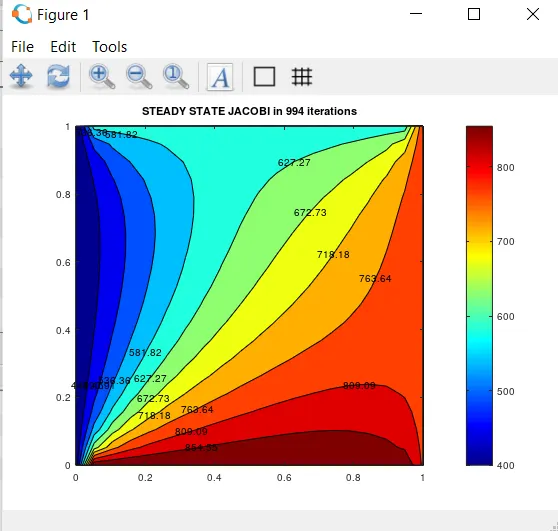
Jacobi method- It is a simplest method,but coes with more problems compared to other methods.It uses predefined values of variable to find new values for each iteration with some permissible error.

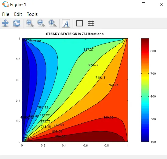
Gauss Seidel- It is modified jacobi method, it uses new values of variable which is updated after each iteraion.

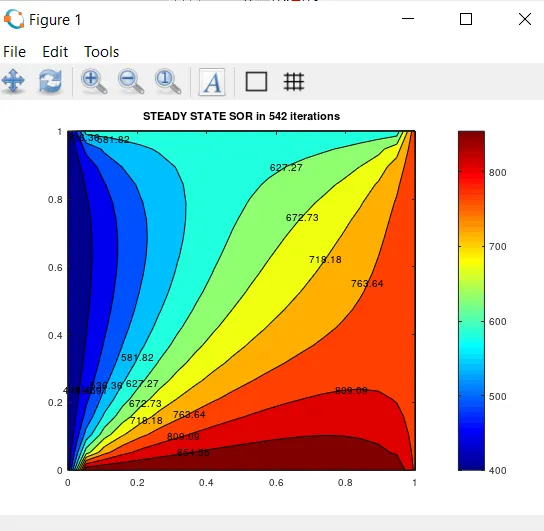
SOR-This method uses a relaxation factor to find new vlaues of variable.

Solution for 2D steady state heat conduction equation.

Ti,j=1/k(T(i-1,j)+T(i+1,j))/`Deltax^2`)+((T(i,j-1)+T(i,j+1))/`Deltay^2`).

k=2(`Deltax^2+Deltay^2`)/`Deltax^2*Deltay^2`

solution for transient state 2D heat conduction equation.

explicit

T^(n+1)i,j=T^n i,j+k1(Ti-1,j-2Ti,j+Ti,j+1)+k2(Ti,j-1-2Ti,j+Ti,j+1)

k1=`alpha*Deltat`/`Deltax^2`

k2=`alpha*Deltat`/`Deltay^2`

Implicit

Ti,j=1/(1+k1+k2) (Ti,j+k1(Ti-1,j+Ti+1,j)+k2(Ti,j-1+Ti,j+1))

CODE EXPLAINATION-

1.A 2D domain is defined is two different variables namely 'nx' , 'ny'.

2.A matrix consisting of temperature values is generated for top, bottom, left and right nodes with help of indexing.

3.Linspace command is used for defining the array of nodes separately for both the variables.

4.Grit spacing between two successive nodes is defined.

5.Variable k which is related to dx and dy, later used in the equations is defined.

6.Error , tolerance and relaxation factor omega for use in SOR method are defied.

7.Solver using input command is used to define type of method i.e jacobi,gs,SOR.

8.Now starting with 'if' to compare input value and method type define the convergence loop and space loop with while statement to compare error and tolerance.

9.Similarly define the loops for gauss seidel and SOR methods and plot the results using contourf command.

MATLAB CODE FOR STEADY STATE HEAT CONDUCTION EQUATION

clear all
close all
clc

% 1d heat conduction equation =d^2x/du^2

nx=20;
ny=nx;

tol=1e-5;
error=1e-4;
x=linspace(0,1,nx);
y=linspace(0,1,ny);
dx=x(2)-x(1);
dy=y(2)-y(1);
t=300*ones(nx,ny);
t(1,:)=600;
t(end,:)=900;
t(:,1)=400;
t(:,end)=800;

k=(2*(dx^2+dy^2)/(dx^2*dy^2));
t_old=t;
t_p=t;

solver=3; % 1.JACOBI 2.GS 3.SOR

%JACOBI METHOD

if solver==1;
  jac_iter=1;
  
  %convergence loop
while (error>tol)
    for i=2:(nx-1);
      for j=2:(ny-1);
        TL=t_old(i-1,j);
        TR=t_old(i+1,j);
        TT=t_old(i,j+1);
        TB=t_old(i,j-1);
        
        H=(TL+TR)/dx^2;
        V=(TT+TB)/dy^2;
        
        t(i,j)=(H+V)/k;
      endfor
    endfor
    error=max(max(abs(t_old-t))); %max(max(A)) reduces 2D array to a single value
    t_old=t;
    jac_iter=jac_iter+1;
end
     
    contourf(x,y,flipud(t),'ShowText','ON'); %flipud flips t upside down as contourf inverts it while plotting
    colormap(jet);
    colorbar;
    title_text=sprintf('STEADY STATE JACOBI in %d iterations',jac_iter);
    title(title_text);   
end

%GAUSS SEIDEL METHOD
 
if solver==2;
  gs_iter=1;
  
  %convergence loop
while (error>tol)
    for i=2:(nx-1);
      for j=2:(ny-1);
        TL=t(i-1,j);  %left is already calculated. Hence GS uses t
        TR=t_old(i+1,j);  
        TT=t(i,j+1);  %top is already calculated. Hence GS uses t
        TB=t_old(i,j-1);
        
        H=(TL+TR)/dx^2;
        V=(TT+TB)/dy^2;
        
        t(i,j)=(H+V)/k;
      endfor
    endfor
    error=max(max(abs(t_old-t))); %max(max(A)) reduces 2D array to a single value
    t_old=t;
    gs_iter=gs_iter+1;
end
     
    contourf(x,y,flipud(t),'ShowText','ON'); %flipud flips t upside down as contourf inverts it while plotting
    colormap(jet);
    colorbar;
    title_text=sprintf('STEADY STATE GS in %d iterations',gs_iter);
    title(title_text);   
end


%SOR METHOD

if solver==3;
  sor_iter=1;
  omega = 1.3; %Relaxation factor for SOR
  %convergence loop
while (error>tol)
    for i=2:(nx-1);
      for j=2:(ny-1);
        TL=t(i-1,j);  %left is already calculated. Hence GS uses t
        TR=t_old(i+1,j);  
        TT=t(i,j+1);  %top is already calculated. Hence GS uses t
        TB=t_old(i,j-1);
        
        H=(TL+TR)/dx^2;
        V=(TT+TB)/dy^2;
        
        t_gs=(H+V)/k;
        t(i,j) = (1-omega)*t_old(i,j) + omega*t_gs; %SOR formulation
      endfor
    endfor
    error=max(max(abs(t_old-t))); %max(max(A)) reduces 2D array to a single value
    t_old=t;
    sor_iter=sor_iter+1;
end
     
    contourf(x,y,flipud(t),'ShowText','ON'); %flipud flips t upside down as contourf inverts it while plotting
    colormap(jet);
    colorbar;
    title_text=sprintf('STEADY STATE SOR in %d iterations',sor_iter);
    title(title_text);   
end

RESULTS FOR STEADY STATE

MATLAB CODE FOR TRANSIENT STATE IMPLICIT FUNCTION

close all
clear all
clc

nx=20;
ny=nx;
alpha=1.4;
tol=1e-5;
error=1e-4;
x=linspace(0,1,nx);
y=linspace(0,1,ny);
T=5;
dt=1e-2
dx=x(2)-x(1);
dy=y(2)-y(1);
t=300*ones(nx,ny);
t(1,:)=600;
t(end,:)=900;
t(:,1)=400;
t(:,end)=800;

k1=alpha*(dt/dx^2);
k2=alpha*(dt/dy^2);
k=1+(2*k1)+(2*k2);
t_old=t;
t_p=t;

solver=3

%JACOBI METHOD

if solver==1;
  jac_iter=1;
  
  %convergence loop
while (error>tol)
    for i=2:(nx-1);
      for j=2:(ny-1);
        TL=t_old(i-1,j);
        TR=t_old(i+1,j);
        TT=t_old(i,j+1);
        TB=t_old(i,j-1);
        
        H=(TL+TR);
        V=(TT+TB);
        
        t(i,j)=(t_p(i,j)+H*k1+V*k2)/k;
      endfor
    endfor
    error=max(max(abs(t_old-t))); %max(max(A)) reduces 2D array to a single value
    t_old=t;
    jac_iter=jac_iter+1;
end
     
    contourf(x,y,flipud(t),'ShowText','ON'); %flipud flips t upside down as contourf inverts it while plotting
    colormap(jet);
    colorbar;
    title_text=sprintf('STEADY STATE JACOBI in %d iterations',jac_iter);
    title(title_text);   
end

%GAUSS SEIDEL METHOD
 
if solver==2;
  gs_iter=1;
  
  %convergence loop
while (error>tol)
    for i=2:(nx-1);
      for j=2:(ny-1);
        TL=t(i-1,j);  %left is already calculated. Hence GS uses t
        TR=t_old(i+1,j);  
        TT=t(i,j+1);  %top is already calculated. Hence GS uses t
        TB=t_old(i,j-1);
        
        H=(t(i-1,j)+TR);
        V=(TT+t(i,j-1));
       t(i,j)=(t_p(i,j)+H*k1+V*k2)/k;
      endfor
    endfor
    error=max(max(abs(t_old-t))); %max(max(A)) reduces 2D array to a single value
    t_old=t;
    gs_iter=gs_iter+1;
end
     
    contourf(x,y,flipud(t),'ShowText','ON'); %flipud flips t upside down as contourf inverts it while plotting
    colormap(jet);
    colorbar;
    title_text=sprintf('STEADY STATE GS in %d iterations',gs_iter);
    title(title_text);   
end


%SOR METHOD

if solver==3;
  sor_iter=1;
  omega = 1.3; %Relaxation factor for SOR
  %convergence loop
while (error>tol)
    for i=2:(nx-1);
      for j=2:(ny-1);
        TL=t(i-1,j);  %left is already calculated. Hence GS uses t
        TR=t_old(i+1,j);  
        TT=t(i,j+1);  %top is already calculated. Hence GS uses t
        TB=t_old(i,j-1);
        
        H=(t(i-1,j)+TR);
        V=(TT+t(i,j-1));
        
        t_gs=(t_p(i,j)+H*k1+V*k2)/k;
        t(i,j) = (1-omega)*t_old(i,j) + omega*t_gs; %SOR formulation
      endfor
    endfor
    error=max(max(abs(t_old-t))); %max(max(A)) reduces 2D array to a single value
    t_old=t;
    sor_iter=sor_iter+1;
end
     
    contourf(x,y,flipud(t),'ShowText','ON'); %flipud flips t upside down as contourf inverts it while plotting
    colormap(jet);
    colorbar;
    title_text=sprintf('STEADY STATE SOR in %d iterations',sor_iter);
    title(title_text);   
end

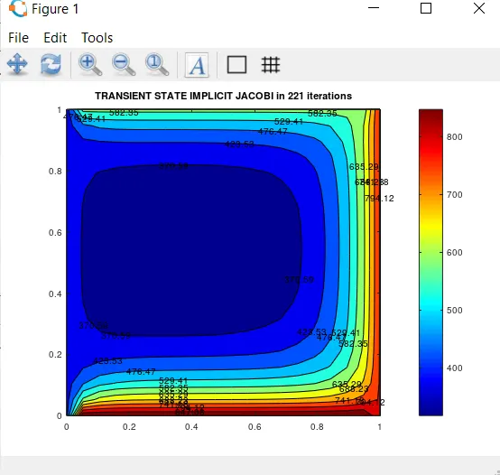
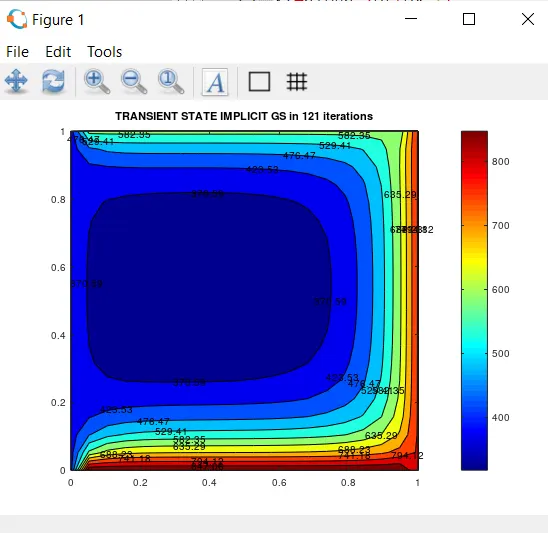
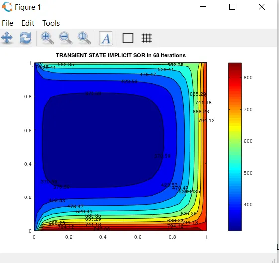
RESULTS FOR TRANSIENT STATE IMPLICIT FUNCTION

MATLAB CODE FOR TRANSIENT STATE EXPLICIT FUNCTION

close all
clear all
clc

nx=20;
ny=nx;
alpha=0.4; %Alpha adjusted to satisfy CFL condition
tol=1e-5;
error=9e9; %time iterative error
x=linspace(0,1,nx);
y=linspace(0,1,ny);
dt=1e-3;
dx=x(2)-x(1);
dy=y(2)-y(1);
t=300*ones(nx,ny);
t(1,:)=600;
t(end,:)=900;
t(:,1)=400;
t(:,end)=800;

k1=alpha*(dt/dx^2);
k2=alpha*(dt/dy^2);
cfl = k1+k2; %Explicit CFL condition <= 0.5
k=1-(2*k1)-(2*k2);
tprev=t; %No iterations, hence no t_old
time_iter = 1; 


%EXPLICIT METHOD (current time unkown is found by previous time)

  %convergence loop
while (error>tol)
    for i=2:(nx-1);
      for j=2:(ny-1);
        TL=tprev(i-1,j);
        TR=tprev(i+1,j);
        TT=tprev(i,j+1);
        TB=tprev(i,j-1);
        
        H=(TL+TR);
        V=(TT+TB);
        
        t(i,j)=(tprev(i,j)*k + H*k1 + V*k2);
      endfor
    endfor
    error=max(max(abs(t-tprev))); %max(max(A)) reduces 2D array to a single value
    tprev=t;
    time_iter = time_iter + 1;
 end   
 contourf(x,y,flipud(t),'ShowText','ON'); %flipud flips t upside down as contourf inverts it while plotting
 colormap(jet);
 colorbar;
 title({['Timestep = ',num2str(dt)],['Thermal diffusivity = ',num2str(alpha)],['CFL = ',num2str(cfl)] ...
 ,['Time iterations = ',num2str(time_iter)]}); 

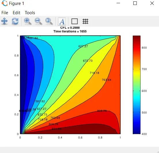
RESULT FOR TRANSIENT STATE EXPLICIT FUNCTION

CONCLUSION-

From the above study it is observed that the SOR method has highest accuracy with least number of iteratios compared to jacobi and gauss seidel method required that the relaxation factor is taken withi the permissible limits.