Week 3.5 - Deriving 4th order approximation of a 2nd order derivative using Taylor Table method

AIM- To derive 4th order approximation of a second order derivative using taylor's table method.

Theory-

Central differencing- nodes=P+Q-1=2+4-1=5

Where, P is order of derivative

Q is order of approximation

Taylor Table for central differencing scheme-

	f(i)	f'(i)`Delta`x	f''(i)`Delta`x^2	f'''(i)`Delta`x^3	f''''(i)`Delta`x^4
af(i-2)	a	-2a	4a/2	-8a/6	16a/24
bf(i-1)	b	-b	b/2	-b/6	b/24
cf(i)	c	0	0	0	0
df(i+1)	d	d	d/2	d/6	d/24
ef(i+2)	e	2e	4e/2	8e/6	16e/24

a+b+c+d+e=0

-2a+(-b)+0+d+2e=0a+b+c+d+e=0

4a/2+b/2+0+d/2+4e/2=1

-8a/6+(-b/6)+0+d/6+8e/6=0

16a/24+b/24+0+b/24+16e/24=0

MATRICES-

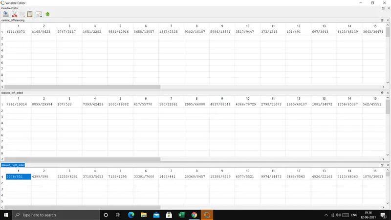
A=[1 1 1 1 1;-2 -1 0 1 2;4/2 1/2 0 1/2 4/2;-8/6 -1/6 0 1/6 8/6;16/24 1/24 0 1/24 16/24]

B=[0;0;1;0;0]

X=[a;b;c;d;e]

X=inv(A)*B

Skewed right sided difference

nodes,N=p+q

p=2

q=4

N=2+4=6

TAYLOR'S TABLE FOR RIGHT SIDED DIFFERENCE

	f(i)	f'(i)`Delta`x	f''(i)`Delta`x^2	f'''(i)`Delta`x^3	f''''(i)`Delta`x^4	f'''''(i)`Delta`x^5
af(i)	a	0	0	0	0	0
bf(i)	b	b	b/2	b/6	b/24	b/120
cf(i)	c	2c	4c/2	8c/6	16c/24	32c/120
df(i)	d	3d	9d/2	27d/6	81d/24	243d/120
ef(i)	e	4e	16e/2	64e/6	256e/24	1024e/120
gf(i)	g	5g	25g/2	125g/6	625g/24	3125g/120

a+b+c+d+e+g=0

0+b+2c+3d+4e+5g=0

0+b/2+4c/2+9d/2+16e/2+25g/2=0

0+b/6+8c/6+27d/6+64e/6+125g/6=0

0+b/24+16c/24+81d/24+256e/24+625g/24=0

0+b/120+32c/120+243d/120+1024e/120+3125g/120=0

A=[1 1 1 1 1 1;0 1 2 3 4 5;0 1/2 4/2 9/2 16/2 25/2;0 1/6 8/6 27/6 64/6 125/6;0 1/24 16/24 81/24 256/24 625/24;0 1/120 32/120 243/120 1024/120 3125/120]

B=[0;0;1;0;0;0]

X=[a;b;c;d;e;g]

X=inv(A)*B

Skewed left sided difference-

nodes,N=p+q

p=2

q=4

N=2+4=6

TAYLOR'S TABLE FOR LEFT SIDED DIFFERENCE

	f(i)	f'(i)`Delta`x	f''(i)`Delta`x^2	f'''(i)`Delta`x^3	f''''(i)`Delta`x^4	f'''''(i)`Delta`x^5
af(i)	a	0	0	0	0	0
bf(i)	b	-b	b/2	-b/6	b/24	-b/120
cf(i)	c	-2c	4c/2	-8c/6	16c/24	-32c/120
df(i)	d	-3d	9d/2	-27d/6	81d/24	-243d/120
ef(i)	e	-4e	16e/2	-64e/6	256e/24	-1024e/120
gf(i)	g	-5g	25g/2	-125g/6	625g/24	-3125g/120

a+b+c+d+e+g=0

0+(-b)+(-2c)+(-3d)+(-4e)+(-5g)=0

0+b/2+4c/2+9d/2+16e/2+25g/2=0

0+(-b/6)+(-8c/6)+(-27d/6)+(-64e/6)+(-125g/6)=0

0+b/24+16c/24+81d/24+256e/24+625g/24=0

0+(-b/120)+(-32c/120)+(-243d/120)+(-1024e/120)+(-3125g/120)=0

Matrices-

A=[1 1 1 1 1 1;0 -1 -2 -3 -4 -5;0 1/2 4/2 9/2 16/2 25/2;0 -1/6 -8/6 -27/6 -64/6 -125/6;0 1/24 16/24 81/24 256/24 625/24;0 -1/120 -32/120 -243/120 -1024/120 -3125/120]

B=[0;0;1;0;0;0]

X=[a;b;c;d;e;g]

X=inv(A)*B

MAIN PROGRAM-

close all
clear all
clc

%input
x=pi/3
dx=linspace(pi/4,pi/4000,20);
for i=1:length(dx);
  
  central_differencing(i)=CD_fourth_order(x,dx(i));
  skewed_right_sided(i)=RS_fourth_order(x,dx(i));
  skewed_left_sided(i)=LS_fourth_order(x,dx(i));
end

%plot
figure(1);
loglog(dx,central_differencing,'marker','o','color','r','linewidth',2);
hold on
loglog(dx, skewed_right_sided,'marker','o','color','k','linewidth',2);
hold on
loglog(dx,skewed_left_sided,'marker','o','color','b','linewidth',2);
xlabel('dx');
ylabel('Absolute error');

FUNCTION CODE FOR CENTRAL DIFFERENCING-

function out=CD_fourth_order(x,dx);
  analytical_derivative=-2*exp(x)*sin(x)
  A=[1 1 1 1 1;-2 -1 0 1 2;4/2 1/2 0 1/2 4/2;-8/6 -1/6 0 1/6 8/6;16/24 1/24 0 16/24 1/24];
  B=[0;0;1;0;0];
  X=inv(A)*B;
  format rat
  term1=(X(1))*(exp(x-(2*dx)))*(cos(x-(2*dx)));
  term2=(X(2))*(exp(x-dx))*(cos(x-dx));
  term3=(X(3))*(exp(x))*(cos(x));
  term4=(X(4))*(exp(x+dx))*(cos(x+dx));
  term5=(X(5))*(exp(x+(2*dx)))*(cos(x+(2*dx)));
  
  central_differencing=(term1+term2+term3+term4+term5)/(dx)^2;
 out=abs(central_differencing-analytical_derivative);
end

FUNCTION CODE FOR SKEWED RIGHT SIDED DIFFERENCE-

function out=RS_fourth_order(x,dx);
  
  analytical_derivative=-2*exp(x)*sin(x);
  A=[1 1 1 1 1 1;0 1 2 3 4 5;0 1/2 4/2 9/2 16/2 25/2;0 1/6 8/6 27/6 64/6 125/6;0 1/24 16/24 81/24 256/24 625/24;0 1/120 32/120 243/120 1024/120 3125/120];
  B=[0;0;1;0;0;0];
  X=inv(A)*B;
  format rat
  term1=(X(1))*(exp(x))*(cos(x));
  term2=(X(2))*(exp(x+dx))*(cos(x+dx));
  term3=(X(3))*(exp(x+(2*dx)))*(cos(x+(2*dx)));
  term4=(X(4))*(exp(x+(3*dx)))*(cos(x+(3*dx)));
  term5=(X(5))*(exp(x+(4*dx)))*(cos(x+(4*dx)));
  term6=(X(6))*(exp(x+(5*dx)))*(cos(x+(5*dx)));
  
  right_side_differencing=(term1+term2+term3+term4+term5+term6)/(dx)^2;
 out=abs(right_side_differencing-analytical_derivative);
  end

FUNCTION CODE FOR SKEWED LEFT SIDED DIFFERENCE-

function  out=LS_fourth_order(x,dx);
  analytical_derivative=-2*exp(x)*sin(x);
  A=[1 1 1 1 1 1;0 -1 -2 -3 -4 -5;0 1/2 4/2 9/2 16/2 25/2;0 -1/6 -8/6 -27/6 -64/6 -125/6;0 1/24 16/24 81/24 256/24 625/24;0 -1/120 -32/120 -243/120 -1024/120 -3125/120];
  B=[0;0;1;0;0;0];
  X=inv(A)*B;
  format rat
  term1=(X(1))*(exp(x))*(cos(x));
  term2=(X(2))*(exp(x-dx))*(cos(x-dx));
  term3=(X(3))*(exp(x-(2*dx)))*(cos(x-(2*dx)));
  term4=(X(4))*(exp(x-(3*dx)))*(cos(x-(3*dx)));
  term5=(X(5))*(exp(x-(4*dx)))*(cos(x-(4*dx)));
  term6=(X(6))*(exp(x-(5*dx)))*(cos(x-(5*dx)));
  
  left_side_differencing=(term1+term2+term3+term4+term5+term6)/(dx)^2;
  out=abs(left_side_differencing-analytical_derivative);
  end

Procedure-

1. Input values of x and dx are defined ,linspace command is used to define the range of dx.

2. Second order analytical derivative is calculated from the analytical function and is defined in the program

3.Function codes for central differencing,skewed left sided and skewed right sided differencing are created and error terms are calculated using abs() command.

4.In the main program a for loop is created to compute error along the length of dx

5.And the respective functions are called out in the for loop.

6.The for loop is then closed and the graph is ploted using loglog command.

7.Required legends and labels are given

RESULTS-

PLOT-

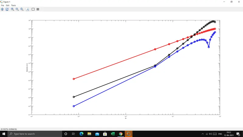
OUT PUT-