Simulation of a 1D Super-sonic nozzle flow simulation using Macormack Method
I. Aim: To simulate the quasi 1D subsonic-supersonic nozzle flow in Matlab using the Macormack Method of numerical solution.
II. Problem Statement:
Simulate the isentropic flow through a quasi 1D subsonic-supersonic nozzle. Derive both the conservation and non-conservation forms of the governing equations and solve them using MacCormack's technique.
1. Determine the steady-state temperature distribution for the flow-field variables and investigate the difference between the two forms of governing equations by comparing their solutions.
2. Report the following plots
a. Steady-state distribution of primitive variables inside the nozzle
b. Time-wise variation of the primitive variables
c. Variation of Mass flow rate distribution inside the nozzle at different time steps during the time-marching process
d. Comparison of Normalized mass flow rate distributions of both forms.
3. Perform a grid independence test on the solution.
III. Theory:
Quasi 1D flow:
A quasi-one-dimensional flow is one in which all flow variables vary primarily along one direction, say x. A flow in a duct with a slowly-varying area A(x) is an example of the quasi 1D flow. In practice this means that the slope of the duct walls is small. Also, the x-velocity component u dominates the y and z-components v and w.
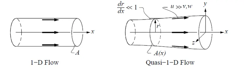
reference: http://web.mit.edu/16.unified/www/SPRING/fluids/Spring2008/LectureNotes/f19.pdf
Isentropic flow through a quasi 1D convergent-divergent nozzle:
Consider a steady isentropic flow through a convergent-divergent nozzle as shown in the below figure:
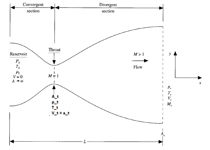
The flow at the inlet comes from a reservoir, where pressure and temperature are denoted by `P_0 and T_0` respectively. The cross-sectional area of the reservoir is large(A---->`oo`), and hence the velocity is small(V--->0). Thus, `P_0 and T_0`are the stagnation values r total pressure and temperatures at the inlet of the nozzle. The flow expands isentropically to supersonic speeds at the exit of nozzle, where exit pressure, temperature, velocity and Mach number are denoted by `p_e, T_e, V_e and M_e`respectively. The flow is locally subsonic in the convergent section, sonic at the throat section(M =1) and supersonic in the divergent section. The area and flow variables at the throat are denoted by `A_t, P_t,V_t,T_t andM_t`. Although the flow properties vary in two dimensions(x and y) in the nozzle, we are assuming a quasi 1D flow throughout the nozzle . This essentially means the flow properties are constant along a cross-section and vary only along the x-direction.
Governing Equations of the flow:
Consider a control volume of length dx along x and cross sectional area dA in the nozzle as shown below:
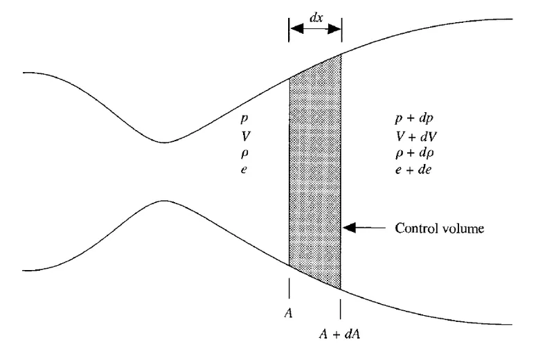
The cross-section area and flow variables at the left and right side of the control volume are shown in the above figure. The governing equations for mass, momentum and energy conservation within the control volume are given by:
Non-Conservation form of Equations:
In the non-conservation method, the control volume under consideration moves along the fluid flow in space and time and the flow passes through it.
1. Continuity Equation:
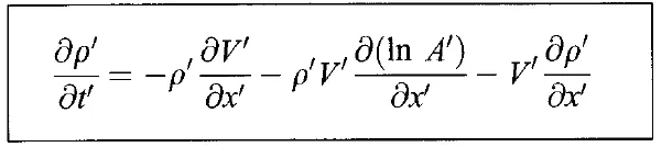
2. Momentum Equation:
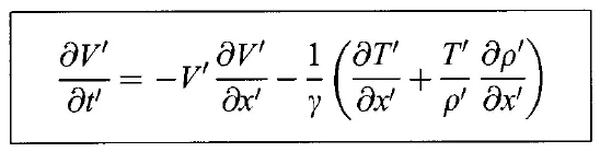
3. Energy Equation:

Conservation form of Equations:
In the conservation method, the control volume under consideration remains fixed in the flow, and the fluid passes through it.
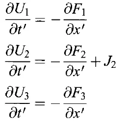
where,
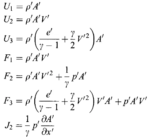
The above eqautions are in the non dimensional form and the non-dimensional form of domain length ,cross-section area, flow properties , time in the above equations defined as follows:
`x' = x/L`;
`A = A/A_t`;
`rho' = rho/rho_0`;
`a_0 = sqrt(gammaRT_0)`;
`v' = v/a_0`;
`p' = p/p_0` ;
`T' = T/T_0`;
`t' = t/(L//a_0)`.
A detailed explanation for the above derivations is given in chapter 7, of Computational Fluid Dynamics the Basics with Applications by John D. Anderson, Jr. textbook.
The above governing equations can be converted into algebraic form by finite difference methods and can be solved by the MacCormack method of the numerical solution.
MacCormack method of the numerical solution:
The MacCormack method is an explicit method of numerical solution which is second-order accurate in both time and space. This method uses a time marching solution with a finite difference method. It consists of a two-step approach namely the predictor step and corrector step in finding the time-dependent flow properties. The flow properties in the predictor step are found by forward difference of space derivatives and the backward difference method in the corrector step. The flow properties from predictor and corrector steps are averaged to find the final flow properties.
In this project, a Matlab program is executed to simulate the quasi 1D isentropic flow through a convegent-divergent nozzle. The non-dimensional governing equations for both conservative and non-conservative form are solved using the MacCormack technique to find the flow properties.
The fluid type, domain properties, initial and boundary conditions for solving the governing equations are taken from chapter 7, of Computational Fluid Dynamics the Basics with Applications by John D. Anderson, Jr. textbook.
IV: Program:
Main Program:
%Isentropic flow simulation through a quasi 1D subsonic-supersonic nozzle.

clear all
close all
clc

%domain description
% L = 3; non dimensional domain length
%grid ponits
n = input(sprintf('Enter the number of grid points = '))';
x = linspace(0,3,n);
dx = x(2)-x(1);

%inputs
%ratio of specific heats , gamma
gamma = 1.4;
%courant number
C = 0.5;
%time steps
nt =1400;

%cross sectional area of nozzle
A = 1+(2.2*(x-1.5).^2);


%nonconservative form of solution
[rho_n,v_n,T_n,p_n,m_n,M_n,rho_tn,v_tn,T_tn,p_tn,m_tn,M_tn] = nonconservative(n,x,dx,nt,C,A,gamma);

   % Time-wise variation of the primitive variables at the nozzle throat
   figure(1)
  %density
  subplot(5,1,1)
  plot(linspace(1,nt,nt),rho_tn,'linewidth',2)
  xlabel('Timestep')
  ylabel('rho/rho_0')
  title('Time-wise variation of the primitive variables at the nozzle throat for nonconservative form')
  %Temperature
  subplot(5,1,2)
  plot(linspace(1,nt,nt),T_tn,'linewidth',2)
  xlabel('Timestep')
  ylabel('T/T_0')
  %Pressure ratio
  subplot(5,1,3)
   plot(linspace(1,nt,nt),p_tn,'linewidth',2)
   xlabel('Timestep')
  ylabel('p/p_0')
  %Mach Number
  subplot(5,1,4)
  plot(linspace(1,nt,nt),M_tn,'linewidth',2)
  xlabel('Timestep')
  ylabel('M')

%conservative form of solution
[rho_c,v_c,T_c,p_c,m_c,M_c,rho_tc,v_tc,T_tc,p_tc,m_tc,M_tc] = conservative(n,x,dx,nt,C,A,gamma);

 %Time-wise variation of the primitive variables at the nozzle throat
   figure(4)
  %density
  subplot(5,1,1)
  plot(linspace(1,nt,nt),rho_tc,'linewidth',2)
  xlabel('Timestep')
  ylabel('rho/rho_0')
  title('Time-wise variation of the primitive variables at the nozzle throat for conservative form')
  %Temperature
  subplot(5,1,2)
  plot(linspace(1,nt,nt),T_tc,'linewidth',2)
  xlabel('Timestep')
  ylabel('T/T_0')
  %Pressure ratio
  subplot(5,1,3)
   plot(linspace(1,nt,nt),p_tc,'linewidth',2)
   xlabel('Timestep')
  ylabel('p/p_0')
  %Mach Number
  subplot(5,1,4)
  plot(linspace(1,nt,nt),M_tc,'linewidth',2)
  xlabel('Timestep')
  ylabel('M')


%comparsion of mass flowrate for nonconservative and conservative form
figure(7)
plot(x,m_n,'linewidth',2)
hold on
plot(x,m_c,'linewidth',2)
xlabel('x/L')
ylabel('(rhovA/rho_0v_0A_t)')
legend('Non-conservative form', 'Conservative form')
title('comparsion of nondimensional mass flowrate for nonconservative and conservative form')
Code explanation:
Step1: clear all – command to clear the workspace.
Step 2: close all – command to close all opened previous plots.
Step 3: clc – command to clear the command window.
Step 4: Defining the domain properties, number of grid points, ratio of specific heats, courant number, number of timesteps and cross-sectional area profile.
Step 5: Calling the function codes for both non-conservative and conservative form of solution. The function codes are given below:
Function code for nonconservative form of solution
%Function code nonconservative form of solution

function [rho_n,v_n,T_n,p_n,m_n,M_n,rho_tn,v_tn,T_tn,p_tn,m_tn,M_tn] = nonconservative(n,x,dx,nt,C,A,gamma)


%initial profiles for nonconservative form
rho_n= 1-(0.3146*x);
T_n= 1-(0.2314*x);
v_n = (0.1+1.09*x).*T_n.^(1/2);


   %timestep calcuLATION
   for i =1:n
     dt(i) = C*(dx/(T_n(i)^(1/2)+v_n(i)));
   end
   dt = min(dt);

   %Time marching loop
   for k = 1:nt
        %initial conditions
    rho_old = rho_n;
    v_old = v_n;
    T_old = T_n;

    %MacCorkmack Method for space loop
    for j =2:n-1
    %predictor step (Forward difference)

    dvdx = (v_n(j+1)-v_n(j))/dx;
    dlogadx = (log(A(j+1))-log(A(j)))/dx;
    drhodx = (rho_n(j+1)-rho_n(j))/dx;
    dTdx = (T_n(j+1)-T_n(j))/dx;

    %continuity equation
    drhodt_p(j) = -rho_n(j)*dvdx-rho_n(j)*v_n(j)*dlogadx-v_n(j)*drhodx;

    %momentum eqaution
    dvdt_p(j) = -v_n(j)*(dvdx)-(1/gamma)*(dTdx+(T_n(j)/rho_n(j)*(drhodx)));

    %Energy equation
    dTdt_p(j) = -v_n(j)*dTdx-((gamma-1)*T_n(j)*(dvdx+v_n(j)*dlogadx));

    %solution update
    rho_n(j) = rho_old(j)+drhodt_p(j)*dt;
    v_n(j) = v_old(j)+dvdt_p(j)*dt;
    T_n(j) = T_old(j)+dTdt_p(j)*dt;
    end
    for j = 2:n-1
    %corrector step(Backward difference)
    dvdx = (v_n(j)-v_n(j-1))/dx;
    dlogadx = (log(A(j))-log(A(j-1)))/dx;
    drhodx = (rho_n(j)-rho_n(j-1))/dx;
    dTdx = (T_n(j)-T_n(j-1))/dx;

    %continuity equation
    drhodt_c(j) = -rho_n(j)*dvdx-rho_n(j)*v_n(j)*dlogadx-v_n(j)*drhodx;

    %momentum eqaution
    dvdt_c(j) = -v_n(j)*(dvdx)-(1/gamma)*(dTdx+(T_n(j)/rho_n(j)*(drhodx)));

    %Energy equation
    dTdt_c(j) = -v_n(j)*dTdx-((gamma-1)*T_n(j)*(dvdx+v_n(j)*dlogadx));

    end

    %average quantities
    drhodt = 0.5*(drhodt_p+drhodt_c);
    dvdt = 0.5*(dvdt_p+dvdt_c);
    dTdt = 0.5*(dTdt_p+dTdt_c);


    for i = 2:n-1
    %Final solution update
    rho_n(i) = rho_old(i)+drhodt(i)*dt;
    v_n(i) = v_old(i)+dvdt(i)*dt;
    T_n(i) = T_old(i)+dTdt(i)*dt;
    end

    %BC
    %inlet
    v_n(1) = 2*v_n(2)-v_n(3);
    %outlet
    rho_n(n) = 2*rho_n(n-1)-rho_n(n-2);
    v_n(n) = 2*v_n(n-1)-v_n(n-2);
    T_n(n) = 2*T_n(n-1)-T_n(n-2);


  %pressure from equation of state (P = rho*T)
  p_n=rho_n.*T_n;
  %massflowrate m = rho*a*v
  m_n= rho_n.*A.*v_n;
  %Mach Number
  M_n = v_n./(T_n.^(1/2));

   %throat position
    x_t = find(A==1);
    %Variable values at Throat
    rho_tn(k) = rho_n(x_t);
    v_tn(k)  = v_n(x_t);
    T_tn(k) = T_n(x_t);
    m_tn(k) = m_n(x_t);
    p_tn(k) = p_n(x_t);
    M_tn(k) = M_n(x_t);


  %plotting maas flowrate with respect to timestep
     if k == 1
        figure(2)
        plot(x,(rho_n.*v_n.*A),'linewidth',2)
        hold on
     end
       if k == 50
        plot(x,(rho_n.*v_n.*A),'linewidth',2)
     end
    if k == 100
        plot(x,(rho_n.*v_n.*A),'linewidth',2)

    end
    if k == 150
        plot(x,(rho_n.*v_n.*A),'linewidth',2)
        legend(sprintf('timestep = %d',k))
    end
    if k == 200
        plot(x,(rho_n.*v_n.*A),'linewidth',2)
        legend(sprintf('timestep = %d',k))
    end
    if k == 700
        plot(x,(rho_n.*v_n.*A),'linewidth',2)
        legend(sprintf('timestep = %d',k))
    end

   end
   %title,axis,legend of figure(1)
    xlabel('Non-dimensional distance through nozzle (x/L)')
    ylabel('Non-dimensional mass flowrate(rhovA/rho_0v_0A_t)')
    title('Instantaneous nondimensional mass flowrate distribution for different time steps for nonconservative form')
    legend('0Deltat','50Deltat','100Deltat','150Deltat','200Deltat','700Deltat')

  %plotting the steady state distribution of primitive variables

  figure(3)
  %density
  subplot(5,1,1)
  plot(x,rho_n,'linewidth',2)
  xlabel('x/L')
  ylabel('rho/rho_0')
  title('Steady-state distribution of primitive variables inside the nozzle for nonconservative form')
  %Temperature
  subplot(5,1,2)
  plot(x,T_n,'linewidth',2)
  xlabel('x/L')
  ylabel('T/T_0')
  %Pressure
  subplot(5,1,3)
  plot(x,p_n,'linewidth',2)
  xlabel('x/L')
  ylabel('p/p_0')
  %Mach Number
  subplot(5,1,4)
  plot(x,M_n,'linewidth',2)
  xlabel('x/L')
  ylabel('M')


end
Function code for nonconservative form of solution
%Function code for conservative form of solution

function [rho_c,v_c,T_c,p_c,m_c,M_c,rho_tc,v_tc,T_tc,p_tc,m_tc,M_tc] = conservative(n,x,dx,nt,C,A,gamma)

  %initial profiles for conservative form

    rho_c = zeros(size(x));
    T_c = zeros(size(x)) ;
    for i = 1:n
        if (0<=x(i))&&(x(i)<=0.5)
        rho_c(i) = 1;
        T_c(i) = 1;
        elseif (0.5<=x(i))&&(x(i)<=1.5)
        rho_c(i) = 1-(0.366*(x(i)-0.5));
        T_c(i) = 1-(0.167*(x(i)-0.5));
        elseif (1.5<=x(i))&&(x(i)<=3.5)
        rho_c(i) =0.634-(0.3879*(x(i)-1.5));
        T_c(i) = 0.833-(0.3507*(x(i)-1.5));
        end
    end
    %mass flow rate across the domain m = 0.59 is assumed
    v_c = 0.59./(rho_c.*A);

    U1=rho_c.*A;
    U2=rho_c.*A.*v_c;
    U3=rho_c.*(T_c./(gamma-1)+(gamma/2)*v_c.^2).*A;

   %timestep calcuLATION
    for i =1:n
     dt(i) = C*(dx/(T_c(i)^(1/2)+v_c(i)));
   end
   dt = min(dt);

   %Time marching loop
    for k =1:nt
    U1_old=U1;
     U2_old=U2;
     U3_old=U3;
    rho_old = U1_old./A;
    v_old = U2_old./U1_old;
    T_old =(gamma-1)*((U3_old./U1_old)-(gamma/2)*v_old.^2);

    %flux terms
     F1 = U2;
     F2=(U2.^2)./U1+((gamma-1)/gamma)*(U3-(gamma/2)*(U2.^2)./U1);
     F3=(gamma*U2.*U3)./U1-((gamma*(gamma-1)/2)*(U2.^3)./U1.^2);

    %MacCormack Method for space loop
    for j = 2:n-1

    %predictor step (Forward difference)

     dadx_p(j) = (A(j+1)-A(j))/dx;
    J2(j) = (1/gamma)*rho_c(j)*T_c(j)*dadx_p(j);
    dF1dx_p(j)= (F1(j+1)-F1(j))/dx;
    dF2dx_p(j) = (F2(j+1)-F2(j))/dx;
    dF3dx_p(j)= (F3(j+1)-F3(j))/dx;

    %continuity equation
    dU1dt_p(j) = -(dF1dx_p(j));

    %momentum eqaution
    dU2dt_p(j) = -(dF2dx_p(j))+J2(j);

    %Energy equation
    dU3dt_p(j) = -(dF3dx_p(j));

    %solution update
    U1(j) = U1_old(j)+dU1dt_p(j)*dt;
    U2(j) = U2_old(j)+dU2dt_p(j)*dt;
    U3(j) = U3_old(j)+dU3dt_p(j)*dt;

    end
     rho_c = U1./A;
    v_c = U2./U1;
    T_c = (gamma-1)*((U3./U1)-((gamma/2)*v_c.^2));

   %updated flux terms
     F1 = U2;
    F2=(U2.^2)./U1+((gamma-1)/gamma)*(U3-(gamma/2)*(U2.^2)./U1);
     F3=(gamma*U2.*U3)./U1-((gamma*(gamma-1)/2)*((U2.^3)./(U1.^2)));

    for j = 2:n-1


    %corrector step(Backward difference)
     dadx_c(j) = (A(j)-A(j-1))/dx;
    J2(j) = (1/gamma)*rho_c(j)*T_c(j)*dadx_c(j);
    dF1dx_c(j) = (F1(j)-F1(j-1))/dx;
    dF2dx_c(j) = (F2(j)-F2(j-1))/dx;
    dF3dx_c(j) = (F3(j)-F3(j-1))/dx;

     %continuity equation
    dU1dt_c(j) = -(dF1dx_c(j));

    %momentum eqaution
    dU2dt_c(j) = -(dF2dx_c(j))+J2(j);

    %Energy equation
    dU3dt_c(j) = -(dF3dx_c(j));

    end

    %average quantities
    dU1dt = 0.5*(dU1dt_p+dU1dt_c);
    dU2dt = 0.5*(dU2dt_p+dU2dt_c);
    dU3dt = 0.5*(dU3dt_p+dU3dt_c);


    for i = 2:n-1
    %Final solution update
    U1(i) = U1_old(i)+dU1dt(i)*dt;
    U2(i) = U2_old(i)+dU2dt(i)*dt;
    U3(i) = U3_old(i)+dU3dt(i)*dt;
    end
    rho_c = U1./A;
    v_c = U2./U1;
    T_c = (gamma-1)*((U3./U1)-((gamma/2)*v_c.^2));

    %BC
    %inlet
    rho_c(1) = 1;
    T_c(1) = 1;
    U1(1) = A(1);
    U2(1)= 2*U2(2)-U2(3);
    v_c(1) = U2(1)/U1(1);
    U3(1) = U1(1)*((T_c(1)/(gamma-1))+((gamma/2)*v_c(1)^2));

    %outlet

    U1(n) = 2*U1(n-1)-U1(n-2);
    U2(n) = 2*U2(n-1)-U2(n-2);
    U3(n) = 2*U3(n-1)-U3(n-2);


   rho_c = U1./A;
    v_c = U2./U1;
    T_c = (gamma-1)*((U3./U1)-((gamma/2)*v_c.^2));


  %non dimensional pressure from equation of state (P = rho*T)
  p_c=rho_c.*T_c;
  %non dimensional massflowrate m = rho*a*v
  m_c = rho_c.*A.*v_c;
  %Mach Number
  M_c = v_c./(T_c.^(1/2));


  %throat position
    x_t = find(A==1);
  %Variable values at Throat
   rho_tc(k) = rho_c(x_t);
   v_tc(k) = v_c(x_t);
   T_tc(k) = T_c(x_t);
   m_tc(k) = m_c(x_t);
   p_tc(k) = p_c(x_t);
   M_tc(k) = M_c(x_t);


 %plotting variables with respect to timestep
   if k == 1
        figure(5)
        plot(x,(rho_c.*v_c.*A),'linewidth',2)
        hold on
   end
     if k == 50
        plot(x,(rho_c.*v_c.*A),'linewidth',2)
    end
    if k == 100
        plot(x,(rho_c.*v_c.*A),'linewidth',2)
    end
     if k == 150
        plot(x,(rho_c.*v_c.*A),'linewidth',2)
    end
    if k == 200
        plot(x,(rho_c.*v_c.*A),'linewidth',2)
    end
    if k == 700
        plot(x,(rho_c.*v_c.*A),'linewidth',2)
    end

    end
      %title,axis,legend of figure(4)
     xlabel('Non-dimensional distance through nozzle (x/L)')
     ylabel('Non-dimensional mass flowrate (rhovA/rho_0v_0A_t)')
     title('Instantaneous nondimensional mass flowrate distribution for different time steps for conservative form')
     legend('0Deltat','50Deltat','100Deltat','150Deltat','200Deltat','700Deltat')


 %plotting the steady state distribution of primitive variables

  figure(6)
  %density
  subplot(5,1,1)
  plot(x,rho_c,'linewidth',2)
  xlabel('x/L')
  ylabel('rho/rho_0')
  title('Steady-state distribution of primitive variables inside the nozzle for conservative form')
  %Temperature
  subplot(5,1,2)
  plot(x,T_c,'linewidth',2)
   xlabel('x/L')
  ylabel('T/T_0')
  %Pressure ratio
  subplot(5,1,3)
  plot(x,p_c,'linewidth',2)
  xlabel('x/L')
  ylabel('p/p_0')
  %Mach Number
  subplot(5,1,4)
  plot(x,M_c,'linewidth',2)
  xlabel('x/L')
  ylabel('M')

end
The above function codes solve the governing equations according to the Maccormack method bot tin conservative and nonconservative forms subject to the domain properties, initial and boundary conditions. The flow variables in the non-dimensional form computed and plotted from the above function codes are discussed below.
IV: Output:
Non-conservative form of solution:
The below results are for the number of grid points considered, n =31, Courant number 0.5 and number of time steps, nt = 1400.
1. Time-wise variation of the primitive variables
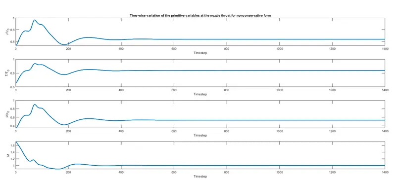
The above plot represents the variation of the non-dimensional flow variables during the time marching solution at the nozzle throat section for the non-conservative form of solution. It can be inferred from the figure that, the solution variables show unsteady nature during the initial stages of the time marching solution process. The variables settle to a steady value after around the 700th time step. Although the solution is run for 1400 time steps, the steady-state reached at around the 700th time step. The Mach number converges to approximately a steady value equal to 1, which confirms that the flow at the throat section of the nozzle is sonic(M=1).
2. Variation of Mass flow rate distribution inside the nozzle at different time steps during the time-marching process
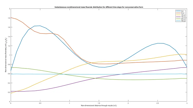
The above figure shows the instantaneous non-dimensional mass flow rate along the nozzle domain at different time step increments. The solution variable varied along the domain length with respect to the initial time step, 50th ,100th ,150th and 200th timestep. But at the time step increment of 700, the mass flowrate attained a stable value of around 0.568 throughout the nozzle length. This represents that the mass is conserved in the domain after the 700th time step.
3. Steady-state distribution of primitive variables inside the nozzle
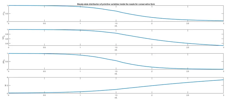
The above figure shows the steady-state distribution of non-dimensional primitive variables inside the nozzle after 700-timestep increments. The density, Temperature and Pressure are non dimensionalized corresponding to the inlet properties. Therefore the values are having a value equal to 1 at the inlet(x/L =0). The values decrease along the nozzle length as the gas are expanding from inlet to exit of the nozzle. But the value of Mach number increases along with the nozzle due to conversion of pressure energy into kinetic energy during the expansion. the value of Mach number increases from inlet to exit, with Mach number less than one (subsonic) in the convergent section of the nozzle(0<= x/L<1.6) and approaches sonic value(M=1) at the throat section (x/L=1.6) and thereafter it increases rapidly in the divergent section (supersonic region).
Conservative form of solution:
The below results are for the number of grid points considered, n =31, Courant number 0.5 and number of time steps, nt = 1400.
1. Time-wise variation of the primitive variables
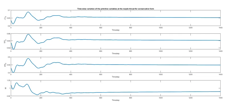
The above plot represents the variation of the non-dimensional flow variables during the time marching solution at the nozzle throat section for the non-conservative form of solution. The results are similar to the non conservative approach results.
2. Variation of Mass flow rate distribution inside the nozzle at different time steps during the time-marching process
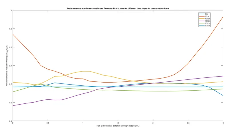
The above figure shows the instantaneous non-dimensional mass flow rate along the nozzle domain at different time step increments. The solution variable varied along the domain length with respect to the initial time step, 50th ,100th ,150th and 200th timestep. But at the time step increment of 700, the mass flowrate attained a stable value of around 0.568 throughout the nozzle length. This represents that the mass is conserved in the domain after the 700th time step.
3. Steady-state distribution of primitive variables inside the nozzle
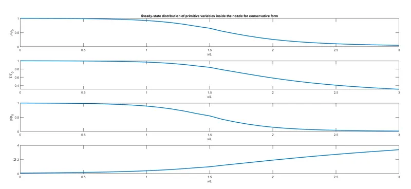
The above figure shows the steady-state distribution of non-dimensional primitive variables inside the nozzle after 700-timestep increments. The density, Temperature and Pressure are non dimensionalized corresponding to the inlet properties. Therefore the values are having a value equal to 1 at the inlet(x/L =0). The values decrease along the nozzle length as the gas are expanding from inlet to exit of the nozzle. But the value of Mach number increases along with the nozzle due to conversion of pressure energy into kinetic energy during the expansion. the value of Mach number increases from inlet to exit, with Mach number less than one (subsonic) in the convergent section of the nozzle(0<= x/L<1.6) and approaches sonic value(M=1) at the throat section (x/L=1.6) and thereafter it increases rapidly in the divergent section (supersonic region).
Comparsion of conservative and non-conservative form of solution:
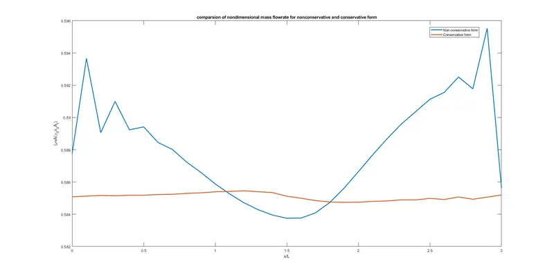
The above figure compares the non dimensuional mass flowrate obtained from the nonconservatve and conservative forms of governing equations after 1400 timesteps (well beyond the convergence timestep of 700 to reach stedy state). The scale of ordinate of massflow rate is greatly magnified to comparre the minute variations in both the forms. It can be predicted that the conservation form of equations provide much more stable mass flow rate result than nonconservation form which has few oscilattions at inlet and exit boundaries.
Table 1: Grid independence study (Throat section results):
| `rho_t/rho_0` | `T_t/T_0` | `p_t/p_0` | `M` | |
|
Exact analytical results |
0.634 | 0.833 | 0.528 | 1.000 |
| Nonconservation form, numerical results (31 grid points) | 0.638 | 0.836 | 0.534 | 0.999 |
| Nonconservation form, numerical results (61 grid points) | 0.637 | 0.835 | 0.532 | 0.999 |
| Nonconservation form, numerical results (91 grid points) | 0.640 | 0.836 | 0.535 | 1.000 |
| Conservation form, numerical results (31 grid points) | 0.652 | 0.841 | 0.548 | 0.978 |
| Conservation form, numerical results (61 grid points) | 0.639 | 0.835 | 0.533 | 0.999 |
| Conservation form, numerical results (91 grid points) | 0.637 | 0.835 | 0.532 | 1.000 |
The grid independence is achieved when the solution doesnt change as we increase the number of grid points. The matter of grid independence is of parmount importance in CFD analysis because, the truncation error in discretization depends on the grid size. For this, a grid independence study is carried out by running the solution with increasing the number of grid points to 61 and 91 . The results of the grid independence study are shown in the above table. It can be seen that the solution variables at the throat section are approaching closer to the analytical results as the grid size is increased for both non conservative and conservative form. But the improvement in the results as grid size is increased from 31 to 61 and 91 is only marginal. Hence we can say that the grid independence is acheived for 31 grid points. The same is true for all locations along the nozzle domain.
Conclusion:
The objective of the project is to simulate a quasi 1D isentropic subsonic-supersonic flow through a convergent-divergent nozzle. The governing equations are solved using Maccorkmack technique for both conservative and nonconservative forms. The following are the conclusions from the curent study:
1. The conservation form yields a better stable mass flow distribution and results in better mass conservation.
2. The results of non conservation form are slightly closer to the analytical results when compared to consevative form. But the results in either case are certainly satisfactory.
3. The grid independence study shows , there is no much variation in results as number of grid points increased above 31.