Simulation of a 1D Super-sonic nozzle flow simulation using MacCormack Method

Simulation of a 1D Super-sonic nozzle flow simulation using MacCormack Method

AIM: To simulate the isentropic flow through a quasi 1D subsonic-supersonic nozzle by deriving the conservation and non-conservation forms of the governing equations and solve them using MacCormack's technique. Also to determine the steady-state temperature distribution for the flow-field variables and investigate the difference between the two forms of governing equations by comparing their solutions.

THEORY:

Derivation of Conservation and Non-Conservation Form of Governing equations for the Isentropic Flow through a 1-D Quasi Subsonic-Supersonic Nozzle

1. Non-Conservation Form:

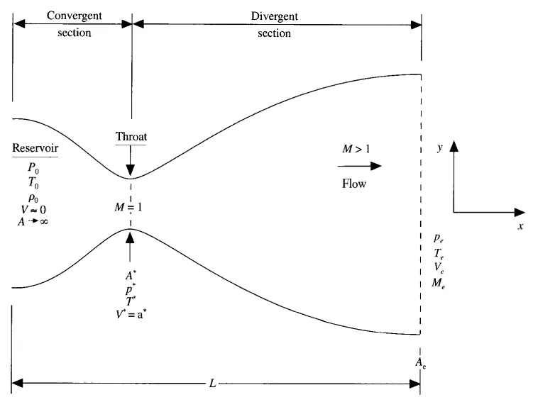
Image 1. Schematic for Subsonic-Supersonic Isentropic Nozzle Flow.

Consider a Steady, Isentropic flow through a convergent-Divergent nozzle as sketched in Image 1. The flow into the nozzle comes from a reservoir where the pressure and temperature are denoted by `p_o` and `T_o`, respectively. The Cross-sectional area of the reservoir is large and hence the velocity is very small. Thus, `p_o` and `T_o` are the stagnation values, or total pressure and total temperature, respectively. The flow expands isentropically to supersonic speeds at the nozzle exit, where the exit pressure, temperature, velocity and Mach number are denoted as `p_e`, `T_e`, `V_e` and `M_e`, respectively. The flow is locally subsonic in the convergent section of the nozzle, sonic at the throat and supersonic at the divergent section of the nozzle. The sonic flow at the throat means that the local velocity at the throat is equal to the local speed of sound. Although the area of the nozzle changes as a function of distance along with the nozzle,x, and therefore, in reality, the flow field is two dimensional, the assumption is made that the flow properties vary only with x, this tantamount to the assuming uniform properties across any given cross-section. Such flow is defined as Quasi 1-D Flow.

The Governing continuity, Momentum and Energy equation for this 1-D, steady, isentropic flow can be expressed as

Continuity: `rho_1V_1A_1 = rho_2V_2A_2`

Momentum: `p_1A_1 + rho_1V_1^2A_1 + int_(A_1)^(A_2)pdA = p_2A_2 + rho_2V_2^2A_2`

Energy: `h_1+V_1^2/2=h_2+V_2^2/2`

Where,

`p = rhoRT` - Perfect Gas Equation

`h = c_pT` - Relation for a Calorifically Perfect Gas

The above equations can be analytically for the flow through the nozzle. Some results are as follows.

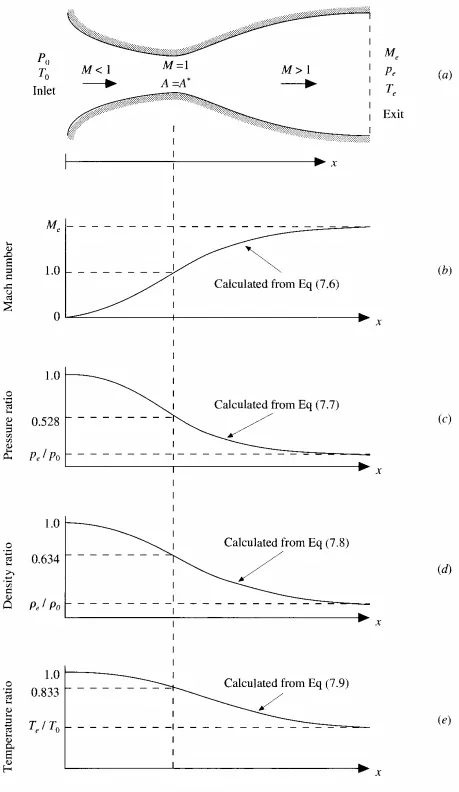
Image 2. Qualitative aspects of Quasi 1-D Nozzle Flow: Isentropic Subsonic-Supersonic solution.

The Setup:

In this section 3 set of equations are calculated for the Time Marching solution Quasi 1-D Subsonic-Supersonic Flow,

1. The governing flow equations will be couched in terms of partial differential equations suitable for the time-Marching solution of quasi 1-D flow.

2. The finite-difference expressions pertaining to MacCormack's Technique as applied to this problem will be set up.

3. Other details for the numerical solution such as the calculation of the time step and the treatment of Boundary Condition is formulated.

1. Governing Equations

The governing flow equations in terms of partial differential equations suitable for the time-marching solution of quasi 1-D flow is shown below in image 3.

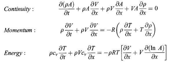
Image 3. Governing flow equations in terms of partial differential equations

The above equations are derived from the Navier-Stokes equations. These equations are taken from the derivation of governing flow equations in terms of partial differential equations suitable for the time-marching solution of quasi 1-D flow in John.D Anderson's Computational Fluid Dynamics-The Basics and Applications.

After deriving these equations, these equations are expressed in terms of Non-Dimensional forms. The Non-Dimensional form of the governing equations are shown below

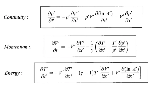
Image 4. Non-Dimensional form of Governing equation.

Non-Dimensional variables vary only from 0 to 1 and this is the aesthetic advantage when presenting the results. And using the finite difference method the discretized form of the governing equations are shown below

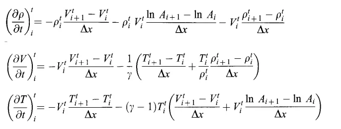
Image 5. Discretized form of the Governing equations.

The solution to these discretized Governing equations is calculated using the MacCormac Method.

MacCormack Method

MacCormack method is a variant of the Lax Wendroff approach but is much simpler in the application. MacCormack approach is an explicit finite-difference technique that is second-order accurate in both space and time. In this method the flow field at each grid point is assumed to be known at the time,`t`, and the flow field variables are calculated at the same grid point at time `t+trianglet` as illustrated in the below figure.

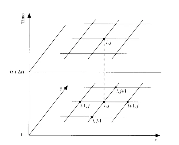
Image 6. A schematic of the grid for Time Marching

For example, to calculate the density at time `t+trianglet`, in the MacCormack method it is obtained as follows

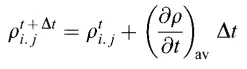
where `((delrho)/(delt))_(av)` is a representative mean value of `(delrho)/(delt)`between the times `t` and `t+trianglet`

The average time derivative, `((delrho)/(delt))_(av)`, is obtained from predictor and corrected philosophy as follows.

1. Predictor Step: In the continuity equation, the spatial derivatives on the RHS is replaced with Forward Differences.

Now, the predicted value of the density, `(overlinerho)^(t+triangleT)`, from the first two terms of the Taylor series, as follows.

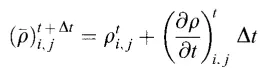
Similarly, the predicted values of the `u`, `v` and `e` are obtained as follows

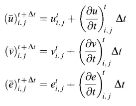
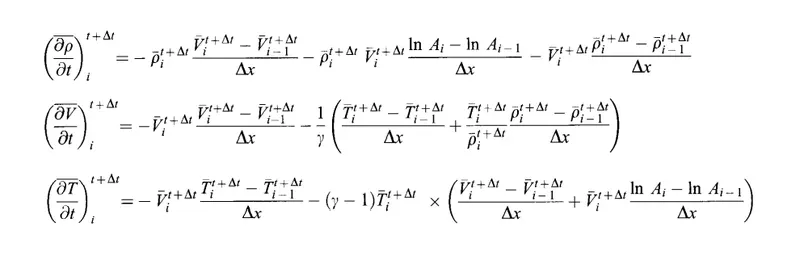
2. Corrected Step: In this step, the predicted value of the time derivative at time,`t+trianglet`, by substituting the predicted values of `rho`, `u`, `v` and `e` into the right side of the continuity equation, replacing the spatial derivative with rearward differences.

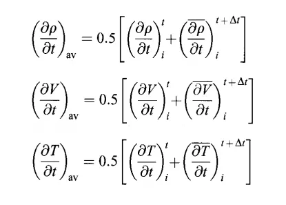
The average value of the time derivative of the density is obtained from the arithmetic mean of `((delrho)/(delt))_(i,j)^t` and `((delrho)/(delt))_(i,j)^(t+trianglet)`

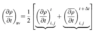
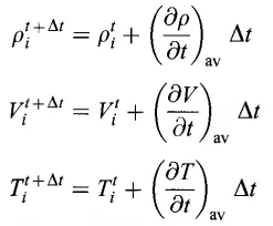
This allows to obtain the correct value of the density at time `t+trianglet` from the below equation

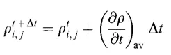
This sequence is repeated at all grid points to obtain the density throughout the flow field at time `t+trianglet`. To calculate `u`, `v` and `e`at time `t+trianglet`, the same technique is used.

The Governing Flow Equation in terms of partial differential equations suitable for the time-marching solution of quasi 1-D flow using the MacCormack Method is shown below

Predictor Step for the Quasi 1-D Subsonic-Supersonic Flow-through Nozzle:

Image 7. Time derivative at time `t` with spatial derivative as Forward Differences.

Predicted values of `rho`,`u`, `v` and `T` are shown below

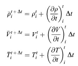
Corrected Step for the Quasi 1-D Subsonic-Supersonic Flow-through Nozzle:

Time derivatives at time `t+trianglet` with spatial derivatives as Backward Differences using the predicted values obtained before.

Average of Time Derivatives

Correct Values of `rho`,`u`, `v` and `T` are obtained from the equations shown below

Boundary Condition:

At the inlet

Velocity at the inlet, `V_1 = 2V_2 - V_3`

Density at the inlet, `rho_1 = 1`

Temperature at the inlet, `T_1 = 1`

At the Outlet

Velocity at the outlet, `V_n = 2V_(n-1) - V_(n-3)`

Density at the outlet, `rho_n = 2rho_(n-1) - rho_(n-3) `

Temeprature at the outlet, `T_n = 2T_(n-1) - T_(n-3)`

Nozzle Shape:

The shape of the nozzle,A = A(x), is specified and held fixed, independent of time. For this case, the section is a parabolic area distribution is used and is given by

`A = 1+2.2(x-1.5)^2`

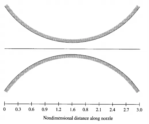
Image 8. Nozzle Profile

Initial Conditions

For this case the initial conditions are as shown below

`rho = 1- 0.3146x`

`T = 1-0.2314x1`

`V = (0.1+1.09x)T^(1/2)`

At `t=0`

Calculation of Mach Number

Mach Number, `M = V/sqrt(T)`

Adaptive Time step:

In the program the Courant Number should be less than 1, and for this program we have selected the Courant Number as 0.5. To keep the Courant Number constant through the program Adaptive time step is used i.e the time step is varied sunch that the Courant Number is always 0.5. The formula for Adaptive Time Step is shown below.

`trianglet = C(trianglex)/(a+V)`

where, a = speed of sound, V= Velocity of flow and C = Courant Number.

All the above equations derived are used in the program to find the solution to the 1-D subsonic-supersonic flow for the nozzle of x/L ratio 3.

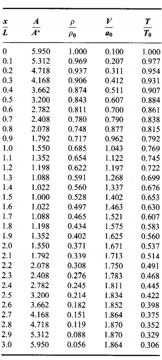
Nozzle Shape and Initial Condition for 31 grid points in the Nozzle is shown below

Intermediate Numerical Results: The First Timestep

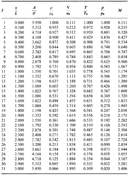
The solution for the first time step is calculated from the equations derived earlier. The below table shows the solution for 31 grid points in the nozzle for the first time step.

Final Numerical Solution: The Steady State solution

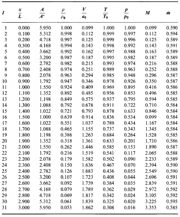
The simulation is run for 1400 time steps to achieve a steady state of flow through the nozzle. The Solutions for the 1-D quasi Subsonic-Supersonic flow at the last time step i.e 1400 time step is shown in the table below.

The Timewise variation of the flow field variables at the nozzle throat where the velocity of the fluid is equal to the speed of sound is shown below.

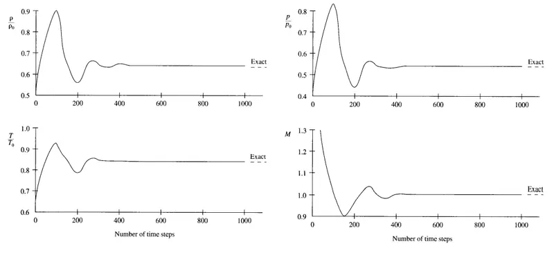
Image 10. Timewise variation of the flow field variables at the nozzle throat

Mass Flow through the Nozzle

The mass flow rate is calculated using the below formula

Mass Flow rate, `dotm = rhoVA`

The mass flow rate will be constant when a steady state is achieved and to find at which time-step the steady-state is achieved the mass flow rate vs nozzle distance is plotted for the different time step. The numerical mass flow rate vs nozzle distance for different time step is shown below.

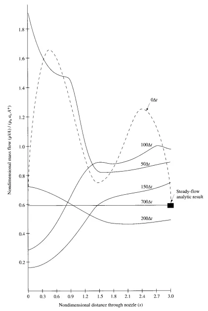
Image 11 Mass flow rate vs nozzle distance for different time step

Conservation Form:

The Conservation form of Governing Equations for the Quasi 1-D Subsonic-Supersonic flow through the nozzle is shown below

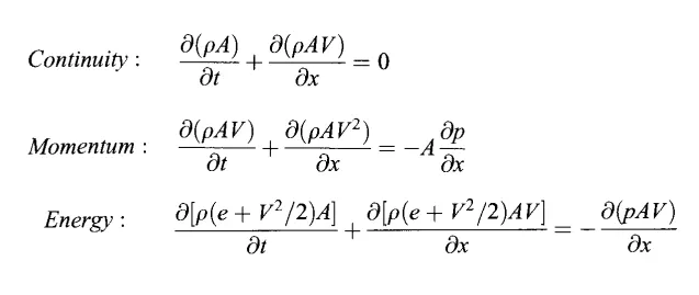
The Non-Dimensional form of the Governing equations for the Quasi 1-D Subsonic-Supersonic flow through the nozzle is shown below

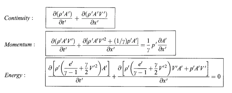
These equations can be expressed in a generic form. Let U be the solution vector, F be the flux vector and the source term be J and as shown below

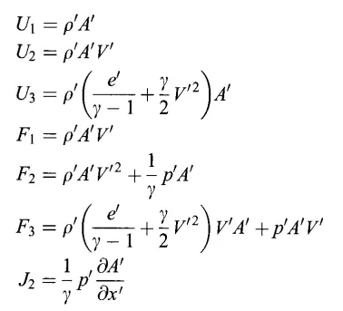
Using these generic form the governing equations are formed and are shown below

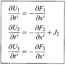
From these solution vectors, the flow field variables are calculated as shown below

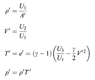
Then the flux vectors are expressed using the solution vectors and are shown below

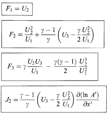
All the Governing equations in the form of solution vector, flux vector and source term are used to find the solution to the Quasi 1-D Subsonic-Supersonic flow through the nozzle.

Predicted Step:

The governing equations for the Predicted Step is shown below

Predicted Time Derivatives using Forward Differencing

`(delU_(1i)^t)/(delt) = (delF_(1i)^t)/(delx)`

`(delU_(2i)^t)/(delt) = (delF_(2i)^t)/(delx)+J_2`

`(delU_(3i)^t)/(delt) = (delF_(3i)^t)/(delx)`

Predicted Solution Vectors

`barU_(1i)^(t+trianglet) = U_(1i)^(t) + (delU_(1i)^t)/(delt)`

`barU_(2i)^(t+trianglet) = U_(2i)^(t) + (delU_(2i)^t)/(delt)`

`barU_(3i)^(t+trianglet) = U_(3i)^(t) + (delU_(3i)^t)/(delt)`

Corrected Step:

In the Corrected step, the Flux Vectors are updated using the same formula derived above using the predicted values calculated in the predicted step. After updating the flux vectors the Correctedted Time derivatives are calculated using the same.

Corrected Time Derivative

`bar(delU_(1i)^t)/(delt) = bar(delF_(1i)^t)/(delx)`

`bar(delU_(2i)^t)/(delt) = bar(delF_(2i)^t)/(delx)+J_2`

`bar(delU_(3i)^t)/(delt) = bar(delF_(3i)^t)/(delx)`

Average Time Derivative:

`((delU_(1i)^(t+trianglet))/(delt))_(avg) = 1/2((delU_(1i)^(t))/(delt) + bar(delU_(1i)^(t+trianglet))/(delt))`

`((delU_(2i)^(t+trianglet))/(delt))_(avg) = 1/2((delU_(2i)^(t))/(delt) + bar(delU_(2i)^(t+trianglet))/(delt))`

`((delU_(3i)^(t+trianglet))/(delt))_(avg) = 1/2((delU_(3i)^(t))/(delt) + bar(delU_(3i)^(t+trianglet))/(delt))`

Corrected Solution Vector

`U_(1i)^(t+trianglet) = U_(1i)^t+((delU_(1i)^(t+trianglet))/(delt))_(avg)`

`U_(2i)^(t+trianglet) = U_(2i)^t+((delU_(2i)^(t+trianglet))/(delt))_(avg)`

`U_(3i)^(t+trianglet) = U_(3i)^t+((delU_(3i)^(t+trianglet))/(delt))_(avg)`

Boundary Condition

Boundary Condition at the Inlet

At the inlet, the two properties are fixed and one property is allowed to float. Below are the equations used to define the inlet boundary condition.

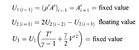
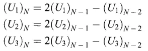
The Outlet Boundary are obtained by linear extrapolation from the two adjacent internal points and equations to calculate the outlet boundary are shown below

Initial Conditions

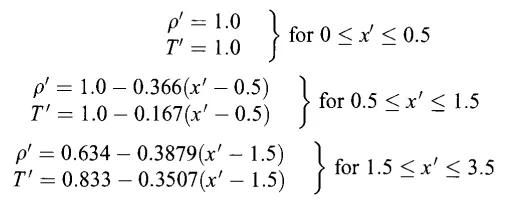
Initial conditions for the solution vector U1, U2 and U3 were synthesized by assuming the following variation of `rho` and `T` and are shown below.

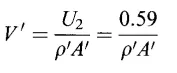
The assumed value of the variation of velocity flow for the Initial condition is shown below.

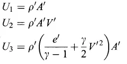
Also, the Solution vector is initially defined using the assumed values of `rho`, `T` and ` V` using the below formula.

Time step is calculated as before i.e as like non-conservation form.

Adaptive Time step:

In the program the Courant Number should be less than 1, and for this program we have selected the Courant Number as 0.5. To keep the Courant Number constant through the program Adaptive time step is used i.e the time step is varied sunch that the Courant Number is always 0.5. The formula for Adaptive Time Step is shown below.

`trianglet = C(trianglex)/(a+V)`

where, a = speed of sound, V= Velocity of flow and C = Courant Number.

Intermediate Calculation: First Time Step

Initial conditions for this case using the Conservation form for 31 grid points through the nozzle is shown below

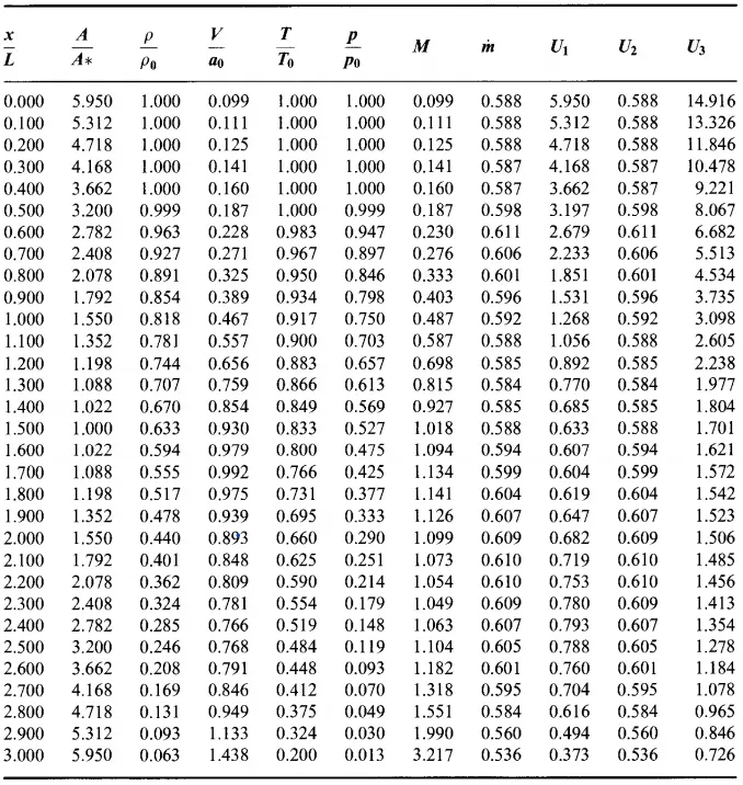
Final Numerical Solution: The Steady State Solution

The simulation is run for 1400 time steps to achieve steady-state of flow through the nozzle. The Solutions for the 1-D quasi Subsonic-Supersonic flow at the last time step i.e 1400 time step is shown in the table below.

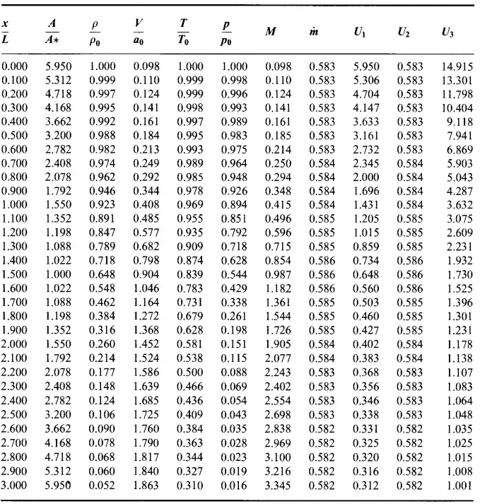
The Timewise variation of the flow field variables at the nozzle throat where the velocity of the fluid is equal to the speed of sound is shown below.

Image 12. Timewise variation of the flow field variables at the nozzle throat

Mass Flow through the Nozzle

The mass flow rate is calculated using the below formula

Mass Flow rate, `dotm = rhoVA`

The mass flow rate will be constant when the steady-state is achieved and to find at which time-step the steady-state is achieved the mass flow rate vs nozzle distance is plotted for the different time step. The numerical mass flow rate vs nozzle distance for different time step is shown below.

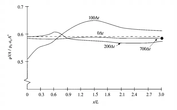
Image 13. Mass flow rate vs nozzle distance for different time step

Comparison of Solution obtained from the Conservation and Non-Conservation from of the Governing Equation is shown below

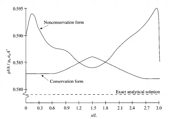
Image 14. Comparison of Solution obtained from the Conservation and Non-Conservation form of the Governing Equation

PROGRAM:

Program to find the Solution for the 1-D Quasi Subsonic-Supersonic, Isentropic Flow through a Nozzle.

The solution for the 1-D quasi Subsonic-Supersonic flow using the Conservation and Non-Conservation form of Governing equation is calculated by developing a program that uses the Discretized equation of the Governing equation and plots the Flowfield variables. Two programs were developed to calculate the solution of governing equation of Conservation and Non-Conservation form and both programs are converted into functions so that another program developed will plot the Comparison of Solution obtained from the Conservation and Non-Conservation form of the Governing Equation. The flow of the program, for both Conservation and Non-conservation form, is as follows

1. Clearing the workspace and command window and closing all the figures.
2. Defining the Initial Conditions.
3. Predictor step.
4. Corrected Step.
5. Boundary Conditions.
6. Calculation of the Flow Field Variables.
7. Updating the Values.
8. Plotting the Mass Flow rate for the different time step.
9. Plotting the graph of Flow Field Variables through the Nozzle.
10. Plotting the Timewise Variation of Flow Field Variable at the throat.

Step 1: Clearing the workspace and command window and closing all the figures.

Below commands are used to clear the workspace and command window and close all the figures.

clear all
close all
clc

Step 2: Defining the Initial Conditions.

The initial condition for the Non-Conservation form of Governing Equation as defined earlier in the derivation is used in the program and is as below syntax.

%% Inputs
n = 31;
x = linspace(0,3,n);
dx = x(2) - x(1);
gamma = 1.4;
T_Ss = [ 1,50,100,150,200,700];
    
% Calculation of Initial Profiles
rho = 1 - 0.3146*x;
T = 1 - 0.2314*x;
V = (0.1 + 1.09*x).*sqrt(T);

% Nozzle Shape as a function of x
A = 1 + 2.2*(x - 1.5).^2;

% Time Step
nt = 1400;
dt = 0.0201;

Step 3: Predicted Step

The predicted and corrected step are inside the time loop and it will run 1400 times. The predicted step derived in the non-Conservation form is shown below

 % Predictor Step
    
    %Clearing the time derivatives for the next time step
    drho_dt_p = zeros(1,n);
    dT_dt_p = zeros(1,n);
    dV_dt_p = zeros(1,n);
    drho_dt_c = zeros(1,n);
    dT_dt_c = zeros(1,n);
    dV_dt_c = zeros(1,n);
    
    % Saving the old value of Flow field variables for further use
    rho_old = rho;
    V_old = V;
    T_old = T;
    
    % Space Loop in Predictor step
    for j = 2:n-1
        
        dV_dx = ( V(j+1) - V(j) )/dx;
        dlnA_dx = ( log(A(j+1)) - log(A(j)) )/dx;
        drho_dx = ( rho(j+1) - rho(j) )/dx;
        dT_dx = ( T(j+1) - T(j) )/dx;
        
        % Continuity Equation 
        drho_dt_p(j) = -rho(j)*dV_dx - rho(j)*V(j)*dlnA_dx - V(j)*drho_dx;
        
        % Momentum Equation
        dV_dt_p(j) = -V(j)*dV_dx - ( 1/gamma )*( dT_dx + (T(j)/rho(j))*(drho_dx) );
        
        % Energy Equation
        dT_dt_p(j) = -V(j)*dT_dx - ( gamma-1 )*T(j)*( dV_dx + V(j)*dlnA_dx );
        
        % Predicted Values
        rho(j) = rho(j) + drho_dt_p(j)*dt;
        V(j) = V(j) + dV_dt_p(j)*dt;
        T(j) = T(j) + dT_dt_p(j)*dt;
        
    end

Step 4: Corrected Step.

The corrected step derived in the non-Conservation form is shown below

% Corrected Step
        
    for j = 2:n-1
        dV_dx = ( V(j) - V(j-1) )/dx;
        dlnA_dx = ( log(A(j)) - log(A(j-1)) )/dx;
        drho_dx = ( rho(j) - rho(j-1) )/dx;
        dT_dx = ( T(j) - T(j-1) )/dx;
        
        % Continuity Equation 
        drho_dt_c(j) = -rho(j)*dV_dx - rho(j)*V(j)*dlnA_dx - V(j)*drho_dx;
        
        % Momentum Equation
        dV_dt_c(j) = -V(j)*dV_dx - ( 1/gamma )*( dT_dx + (T(j)/rho(j))*(drho_dx) );
        
        % Energy Equation
        dT_dt_c(j) = -V(j)*dT_dx - ( gamma-1 )*T(j)*( dV_dx + V(j)*dlnA_dx );
    end

    % Calculation of Average of Time Derivatives
    drho_dt_avg = 0.5*(drho_dt_p + drho_dt_c);
    dV_dt_avg = 0.5*(dV_dt_p + dV_dt_c);
    dT_dt_avg = 0.5*(dT_dt_p + dT_dt_c);
    
    % Corrected Values
    rho_c = rho_old + drho_dt_avg*dt;
    V_c = V_old + dV_dt_avg*dt;
    T_c = T_old + dT_dt_avg*dt;
    

Step 5: Boundary Conditions.

The Boundary Conditions derived earlier, are applied at the end of the Solution before calculating the flow field variables and the syntax for applying the Boundary Condition is as below

% Applying The Boundary Condition
    V_c(1) = 2*V_c(2) - V_c(3);
        
    rho_c(31) = 2*rho_c(30) - rho_c(29);
    V_c(31) = 2*V_c(30) - V_c(29);
    T_c(31) = 2*T_c(30) - T_c(29);
   

Step 6: Calculation of the Flow Field Variables.

The Below syntax is used to calculate the Flow Field Variables after applying the Boundary Conditions.

    % Pressure Ratio
    p_c = rho_c.*T_c;
    
    % Mach Number
    M = V_c./sqrt(T_c);
    
    % Storing the values at point 16
    rho_16(t_s) = rho_c(16);
    p_16(t_s) = p_c(16);
    T_16(t_s) = T_c(16);
    M_16(t_s) = M(16);
    
    % Non Dimesional Mass Flow
    m_dot = rho.*V.*A;

Step 7: Updating the Values.

The below syntax is used to update the values after calculating the flow field variables.

    % Updating the Values
    rho = rho_c;
    V = V_c;
    T = T_c;

Step 8: Adaptive Time Step

In the program the Courant Number should be less than 1, and for this program we have selected the Courant Number as 0.5. To keep the Courant Number constant through the program Adaptive time step is used i.e the time step is varied sunch that the Courant Number is always 0.5. The formula for Adaptive Time Step used in the program is shown below.

% Adaptive Time Step
dt = min(0.5*dx./(T.^(1/2) + V));

Step 9: Plotting the Mass Flow rate for the different time step.

The Mass Flow rate through the Nozzle is to be calculated at different time step and hence is added inside the time loop. The syntax is used to plot the same is shown below

    %% Plotting the Instantaneous Distribution of Nondimensional Mass as a function of distance through Nozzle at 6 different times
    figure(1)
    for g = 1:length(T_Ss)
        if (t_s == T_Ss(g)) == 1
            plot(x,m_dot,'linewidth',2)
            title('Instantaneous Distribution of Nondimensional Mass as a function of distance through Nozzle at 6 different times','fontsize',16)
            xlabel('Nondimesional Distance through nozzle','fontsize',16)
            ylabel('Nondimensional mass flow','fontsize',16)
            legend('Time step = 1','Time step = 50','Time step = 100','Time step = 150','Time step = 200','Time step = 700','fontsize',16)
            hold on
        end
    end

In the above syntax, 'if' loop is used to provide a condition such that it will plot only for a particular time step and it is inside the 'for' loop to compare the time step number with the time step values for which the plot is to be created is defined in an array in the beginning. The 'hold on' command is used so that it will plot in the same figure.

Step 10: Plotting the graph of Flow Field Variables through the Nozzle.

The below syntax is used to plot the Flow Field Variables through the Nozzle distance is shown below.

%% Plotting the graphs
% Plot 1. Quantitaive aspects of the 1-D flow
% Nozzle Profile
fig_1 = ('Quantitaive aspects of the 1-D flow');
figure('Name',fig_1,'NumberTitle','off')
subplot(5,1,1)
title('Nozzle Shape','fontsize',16)
plot(x,A/2,'b', 'linewidth',3)
hold on
plot(x,-A/2,'b', 'linewidth',3)
str = {'M = 1','A = A^*'};
str_1 = {'P_o','T_o','Inlet'};
str_2 = {'M < 1','M > 1'};
str_3 = {'M_e','P_e','T_e'};
text(1.5,2,str)
text(0.1,0,str_1)
text(1,2,str_2(1))
text(2,2,str_2(2))
text(2.9,0,str_3)
text(2.8,0,'Outlet')

% Variation of Flow Velocity
subplot(5,1,2);
plot(x,M,'r', 'linewidth',2)
title('Variation of Flow Velocity(Mach Number) through the Nozzle','fontsize',16)
ylabel('Mach Number','fontsize',14)

% Variation of Pressure Ratio through the Nozzle
subplot(5,1,3);
plot(x,p_c,'r', 'linewidth',2)
title('Variation of Pressure Ratio through the Nozzle','fontsize',16)
ylabel('Pressure Ratio','fontsize',14)

% Variation of Density through the Nozzle
subplot(5,1,4);
plot(x,rho_c,'r', 'linewidth',2)
title('Variation of Density through the Nozzle','fontsize',16)
ylabel('Density Raio','fontsize',14)

% Variation of Temperature though the Nozzle
subplot(5,1,5);
plot(x,T_c,'r','linewidth',2)
title('Variation of Temperature though the Nozzle','fontsize',16)
ylabel('Temprature Ratio','fontsize',14)

%% Plot 2. Timewise Variation of the parameters at node 16 where A = 1

fig_2 = ('Timewise Variation of the parameters at node 16 where A = 1');
figure('Name',fig_2,'NumberTitle','off')

The above syntax will plot all the graph in the same figure as the subplot is used and in the first subplot, the nozzle profile is created.

Step 11: Plotting the Timewise Variation of Flow Field Variable at the throat.

The below syntax is used to plot the Timewise Variation of Flow Field Variable at the throat.

q = 1:nt; % An array which stores number from 1 to 1400.

% Timewise Varation of Density at node 16 where A = 1
subplot(4,1,1)
plot(q,rho_16, 'r', 'linewidth',2)
ylabel('Density Raio','fontsize',14)
title('Timewise Varation of Density at node 16 where A = 1','fontsize',16)

% Timewise Varation of Temperature at node 16 where A = 1
subplot(4,1,2)
plot(q,T_16, 'r', 'linewidth',2)
ylabel('Temprature Ratio','fontsize',14)
title('Timewise Varation of Temperature at node 16 where A = 1','fontsize',16)

% Timewise Varation of Pressure at node 16 where A = 1
subplot(4,1,3)
plot(q, p_16, 'r', 'linewidth',2)
ylabel('Pressure Ratio','fontsize',14)
title('Timewise Varation of Pressure at node 16 where A = 1','fontsize',16)

% Timewise Varation of Mach Number at node 16 where A = 1
subplot(4,1,4)
plot(q,M_16, 'r', 'linewidth',2)
ylabel('Mach Number','fontsize',14)
xlabel('Number of Time Step','fontsize',14)
title('Timewise Varation of Mach Number at node 16 where A = 1','fontsize',16)

figure(4)
plot(x,m_dot)
axis([0 3 0.58 0.6])

THE COMPLETE PROGRAM:

Non-Conservation Form of Governing equation for the Quasi 1-D Subsonic-Supersonic, Isentropic flow through Nozzle:

clear all
close all
clc


%% Inputs
n = 31;
x = linspace(0,3,n);
dx = x(2) - x(1);
gamma = 1.4;
T_Ss = [ 1,50,100,150,200,700];
    
% Calculation of Initial Profiles
rho = 1 - 0.3146*x;
T = 1 - 0.2314*x;
V = (0.1 + 1.09*x).*sqrt(T);

% Nozzle Shape as a function of x
A = 1 + 2.2*(x - 1.5).^2;

% Time Step
nt = 1400;
dt = 0.0201;

%% CFD Solution of Subsonic-Supersonic Isentropic Nozzle Flow using Macormack Technique
for t_s = 1:nt              % Time Loop
    
    % Space Loop
    
    % Predictor Step
    

    drho_dt_p = zeros(1,n);
    dT_dt_p = zeros(1,n);
    dV_dt_p = zeros(1,n);
    drho_dt_c = zeros(1,n);
    dT_dt_c = zeros(1,n);
    dV_dt_c = zeros(1,n);
    
    rho_old = rho;
    V_old = V;
    T_old = T;
    
    for j = 2:n-1
        
        dV_dx = ( V(j+1) - V(j) )/dx;
        dlnA_dx = ( log(A(j+1)) - log(A(j)) )/dx;
        drho_dx = ( rho(j+1) - rho(j) )/dx;
        dT_dx = ( T(j+1) - T(j) )/dx;
        
        % Continuity Equation 
        drho_dt_p(j) = -rho(j)*dV_dx - rho(j)*V(j)*dlnA_dx - V(j)*drho_dx;
        
        % Momentum Equation
        dV_dt_p(j) = -V(j)*dV_dx - ( 1/gamma )*( dT_dx + (T(j)/rho(j))*(drho_dx) );
        
        % Energy Equation
        dT_dt_p(j) = -V(j)*dT_dx - ( gamma-1 )*T(j)*( dV_dx + V(j)*dlnA_dx );
        
        % Predicted Values
        rho(j) = rho(j) + drho_dt_p(j)*dt;
        V(j) = V(j) + dV_dt_p(j)*dt;
        T(j) = T(j) + dT_dt_p(j)*dt;
        
    end
    
    % Corrected Step
        
    for j = 2:n-1
        
        dV_dx = ( V(j) - V(j-1) )/dx;
        dlnA_dx = ( log(A(j)) - log(A(j-1)) )/dx;
        drho_dx = ( rho(j) - rho(j-1) )/dx;
        dT_dx = ( T(j) - T(j-1) )/dx;
        
        % Continuity Equation 
        drho_dt_c(j) = -rho(j)*dV_dx - rho(j)*V(j)*dlnA_dx - V(j)*drho_dx;
        
        % Momentum Equation
        dV_dt_c(j) = -V(j)*dV_dx - ( 1/gamma )*( dT_dx + (T(j)/rho(j))*(drho_dx) );
        
        % Energy Equation
        dT_dt_c(j) = -V(j)*dT_dx - ( gamma-1 )*T(j)*( dV_dx + V(j)*dlnA_dx );
        
        
    end

    % Calculation of Average of Time Derivatives
    drho_dt_avg = 0.5*(drho_dt_p + drho_dt_c);
    dV_dt_avg = 0.5*(dV_dt_p + dV_dt_c);
    dT_dt_avg = 0.5*(dT_dt_p + dT_dt_c);
    
    
    % Corrected Values
    rho_c = rho_old + drho_dt_avg*dt;
    V_c = V_old + dV_dt_avg*dt;
    T_c = T_old + dT_dt_avg*dt;
    
    % Applying The Boundary Condition
    V_c(1) = 2*V_c(2) - V_c(3);
        
    rho_c(31) = 2*rho_c(30) - rho_c(29);
    V_c(31) = 2*V_c(30) - V_c(29);
    T_c(31) = 2*T_c(30) - T_c(29);
    
    % Pressure Ratio
    p_c = rho_c.*T_c;
    
    % Mach Number
    M = V_c./sqrt(T_c);
    
    % Storing the values at point 16
    rho_16(t_s) = rho_c(16);
    p_16(t_s) = p_c(16);
    T_16(t_s) = T_c(16);
    M_16(t_s) = M(16);
    
    
    % Updating the Values
    rho = rho_c;
    V = V_c;
    T = T_c;
    
    % Non Dimesional Mass Flow
    m_dot = rho.*V.*A;
    % Adaptive Time Step
    dt = min(0.5*dx./(T.^(1/2) + V));
    
    %% Plotting the Instantaneous Distribution of Nondimensional Mass as a function of distance through Nozzle at 6 different times
    figure(1)
    for g = 1:length(T_Ss)
        if (t_s == T_Ss(g)) == 1
            plot(x,m_dot,'linewidth',2)
            title('Instantaneous Distribution of Nondimensional Mass as a function of distance through Nozzle at 6 different times','fontsize',16)
            xlabel('Nondimesional Distance through nozzle','fontsize',16)
            ylabel('Nondimensional mass flow','fontsize',16)
            legend('Time step = 1','Time step = 50','Time step = 100','Time step = 150','Time step = 200','Time step = 700','fontsize',16)
            hold on
        end
    end
end



%% Plotting the graphs
% Plot 1. Quantitaive aspects of the 1-D flow
% Nozzle Profile
fig_1 = ('Quantitaive aspects of the 1-D flow');
figure('Name',fig_1,'NumberTitle','off')
subplot(5,1,1)
title('Nozzle Shape','fontsize',16)
plot(x,A/2,'b', 'linewidth',3)
hold on
plot(x,-A/2,'b', 'linewidth',3)
str = {'M = 1','A = A^*'};
str_1 = {'P_o','T_o','Inlet'};
str_2 = {'M < 1','M > 1'};
str_3 = {'M_e','P_e','T_e'};
text(1.5,2,str)
text(0.1,0,str_1)
text(1,2,str_2(1))
text(2,2,str_2(2))
text(2.9,0,str_3)
text(2.8,0,'Outlet')

% Variation of Flow Velocity
subplot(5,1,2);
plot(x,M,'r', 'linewidth',2)
title('Variation of Flow Velocity(Mach Number) through the Nozzle','fontsize',16)
ylabel('Mach Number','fontsize',14)

% Variation of Pressure Ratio through the Nozzle
subplot(5,1,3);
plot(x,p_c,'r', 'linewidth',2)
title('Variation of Pressure Ratio through the Nozzle','fontsize',16)
ylabel('Pressure Ratio','fontsize',14)

% Variation of Density through the Nozzle
subplot(5,1,4);
plot(x,rho_c,'r', 'linewidth',2)
title('Variation of Density through the Nozzle','fontsize',16)
ylabel('Density Raio','fontsize',14)

% Variation of Temperature though the Nozzle
subplot(5,1,5);
plot(x,T_c,'r','linewidth',2)
title('Variation of Temperature though the Nozzle','fontsize',16)
ylabel('Temprature Ratio','fontsize',14)

%% Plot 2. Timewise Variation of the parameters at node 16 where A = 1

fig_2 = ('Timewise Variation of the parameters at node 16 where A = 1');
figure('Name',fig_2,'NumberTitle','off')

q = 1:nt;

% Timewise Varation of Density at node 16 where A = 1
subplot(4,1,1)
plot(q,rho_16, 'r', 'linewidth',2)
ylabel('Density Raio','fontsize',14)
title('Timewise Varation of Density at node 16 where A = 1','fontsize',16)

% Timewise Varation of Temperature at node 16 where A = 1
subplot(4,1,2)
plot(q,T_16, 'r', 'linewidth',2)
ylabel('Temprature Ratio','fontsize',14)
title('Timewise Varation of Temperature at node 16 where A = 1','fontsize',16)

% Timewise Varation of Pressure at node 16 where A = 1
subplot(4,1,3)
plot(q, p_16, 'r', 'linewidth',2)
ylabel('Pressure Ratio','fontsize',14)
title('Timewise Varation of Pressure at node 16 where A = 1','fontsize',16)

% Timewise Varation of Mach Number at node 16 where A = 1
subplot(4,1,4)
plot(q,M_16, 'r', 'linewidth',2)
ylabel('Mach Number','fontsize',14)
xlabel('Number of Time Step','fontsize',14)
title('Timewise Varation of Mach Number at node 16 where A = 1','fontsize',16)

Conservation Form of Governing equation for the Quasi 1-D Subsonic-Supersonic, Isentropic flow through Nozzle:

clear all
close all
clc


% Inputs
n = 31;
x = linspace(0,3,n);
dx = x(2) - x(1);
gamma = 1.4;


% Time Step
nt = 1400;
dt = 0.0267;
T_Ss = [ 1,50,100,150,200,700];

% Calculation of Initial Profiles
rho = ones(1,n);
T = rho;
for k = 1:n
    if (x(k) >= 0.5) && (x(k) <= 1.5) 
        
        rho(k) = 1 - 0.366*(x(k) - 0.5);
        T(k) = 1 - 0.167*(x(k) - 0.5);
    
    elseif (x(k) >= 1.5) && (x(k) <= 3)
    
        rho(k) = 0.634 - 0.3879*(x(k) - 1.5);
        T(k) = 0.833 - 0.3507*(x(k) - 1.5);
        
    end
end

e = T;

% Nozzle Shape as a function of x
A = 1 + 2.2*(x - 1.5).^2;

% Solution Vectors
U1 = rho.*A;
U2 = 0.59 * ones(1,n);
U3 = rho.*A.*( (e/(gamma-1)) + gamma*0.5*(U2./U1).^2 );

V = U2./(rho.*A);

% Mass Flow rate
m_dot = rho.*A.*V;


for t_s = 1:nt
    
    % Updating the values
    U1_old = U1;
    U2_old = U2;
    U3_old = U3;
    
    [F1 F2 F3] = F_123(U1,U2,U3);
    
    % Space Loop
    % Predictor Step
    
    % J2
    for k = 2:n-1
        
        dlnA_dx = (A(k+1)-A(k))/dx;
        J2(k) = (1/gamma) * ( rho(k)*T(k) )*(dlnA_dx);
 
    % Predicted Time Derivative
        dU1_dt(k) = -(F1(k+1) - F1(k))/dx;
        dU2_dt(k) = -(F2(k+1) - F2(k))/dx + J2(k);
        dU3_dt(k) = -(F3(k+1) - F3(k))/dx;

    % Predicted values of U_1,U_2 and U_3
        U1(k) = U1(k) + dU1_dt(k)*dt;
        U2(k) = U2(k) + dU2_dt(k)*dt;
        U3(k) = U3(k) + dU3_dt(k)*dt;
    end

    % Predicted Value of rho
    rho = U1./A;
    
    % Velocity
    V = U2./U1;
    
    % Temperature
    T = (gamma-1)*( (U3./U1) - (gamma/2) * V.^2 );
       
    % Predicted Fluxes
    [F1 F2 F3] = F_123(U1,U2,U3);
   
        
    for k = 2:n-1
        dlnA_dx = (A(k)-A(k-1))/dx;
        J2(k) = (1/gamma) * ( rho(k)*T(k) )*(dlnA_dx);
    end

    % Corrected Step 

    for k = 2:n-1
        
    % Corrected Time Derivatives
        dU1_dt_c(k) = -(F1(k) - F1(k-1))/dx;
        dU2_dt_c(k) = -(F2(k) - F2(k-1))/dx + J2(k);
        dU3_dt_c(k) = -(F3(k) - F3(k-1))/dx;

    % Average Time Derivative
        dU1_dt_avg(k) = 0.5*( dU1_dt(k) + dU1_dt_c(k) );
        dU2_dt_avg(k) = 0.5*( dU2_dt(k) + dU2_dt_c(k) );
        dU3_dt_avg(k) = 0.5*( dU3_dt(k) + dU3_dt_c(k) );

    % Corrected values of U_1,U_2 and U_3
        U1(k) = U1_old(k) + dU1_dt_avg(k)*dt;
        U2(k) = U2_old(k) + dU2_dt_avg(k)*dt;
        U3(k) = U3_old(k) + dU3_dt_avg(k)*dt;

    end
    
    % Boundary Condition
    U1(1) = A(1);
    U2(1) = 2*U2(2) - U2(3);
    U3(1) = U1(1)*( (T(1)/(gamma-1)) + (gamma*0.5)*(V(1))^2 );
    
    U1(n) = 2*U1(n-1) - U1(n-2);
    U2(n) = 2*U2(n-1) - U2(n-2);
    U3(n) = 2*U3(n-1) - U3(n-2);

    % Corrected Values
    % Rho
    rho = U1./A;
    rho_16(t_s) = rho(16);      % Storing Density Value at node 16 for every Time step
    % Velocity
    V = U2./U1;
    V_16(t_s) = V(16);          % Storing Velocity at node 16 for every Time step
    % Mass Flow
    m_dot = rho.*V.*A;
    % Temperature
    T = (gamma-1)*( (U3./U1) - (gamma/2) * V.^2 );
    T_16(t_s) = T(16);          % Storing Temperature at node 16 for every Time step
    % Pressure
    p = rho.*T;
    p_16(t_s) = p(16);          % Storing Pressure at node 16 for every Time step
    % Mach Number
    M = V./sqrt(T);
    M_16(t_s) = M(16);          % Storing Mach Number at node 16 for every Time step
    % Energy
    e = T;
    % Mass Flow
    m_dot = rho.*V.*A;
    % Adaptive Time Step
    dt = min(0.5*dx./(T.^(1/2) + V));
    
        %% Plotting the Instantaneous Distribution of Nondimensional Mass as a function of distance through Nozzle at 6 different times
    figure(1)
    for g = 1:length(T_Ss)
        if (t_s == T_Ss(g)) == 1
            plot(x,m_dot,'linewidth',2)
            title('Instantaneous Distribution of Nondimensional Mass as a function of distance through Nozzle at 6 different times','fontsize',16)
            xlabel('Nondimesional Distance through nozzle','fontsize',16)
            ylabel('Nondimensional mass flow','fontsize',16)
            legend('Time step = 1','Time step = 50','Time step = 100','Time step = 150','Time step = 200','Time step = 700','fontsize',16)
            hold on
        end
    end
end


% Plotting the graphs
% Plot 1. Quantitaive aspects of the 1-D flow
% Nozzle Profile
fig_1 = ('Quantitaive aspects of the 1-D flow');
figure('Name',fig_1,'NumberTitle','off')
subplot(5,1,1)
title('Nozzle Shape','fontsize',16)
plot(x,A/2,'b', 'linewidth',3)
hold on
plot(x,-A/2,'b', 'linewidth',3)
str = {'M = 1','A = A^*'};
str_1 = {'P_o','T_o','Inlet'};
str_2 = {'M < 1','M > 1'};
str_3 = {'M_e','P_e','T_e'};
text(1.5,2,str)
text(0.1,0,str_1)
text(1,2,str_2(1))
text(2,2,str_2(2))
text(2.9,0,str_3)
text(2.8,0,'Outlet')

% Variation of Flow Velocity
subplot(5,1,2);
plot(x,M,'r', 'linewidth',2)
title('Variation of Flow Velocity(Mach Number) through the Nozzle','fontsize',16)
ylabel('Mach Number','fontsize',14)

% Variation of Pressure Ratio through the Nozzle
subplot(5,1,3);
plot(x,p,'r', 'linewidth',2)
title('Variation of Pressure Ratio through the Nozzle','fontsize',16)
ylabel('Pressure Ratio','fontsize',14)

% Variation of Density through the Nozzle
subplot(5,1,4);
plot(x,rho,'r', 'linewidth',2)
title('Variation of Density through the Nozzle','fontsize',16)
ylabel('Density Raio','fontsize',14)

% Variation of Temperature though the Nozzle
subplot(5,1,5);
plot(x,T,'r','linewidth',2)
title('Variation of Temperature though the Nozzle','fontsize',16)
ylabel('Temprature Ratio','fontsize',14)


% Plot 2. Timewise Variation of the parameters at node 16 where A = 1

fig_2 = ('Timewise Variation of the parameters at node 16 where A = 1');
figure('Name',fig_2,'NumberTitle','off')

q = 1:nt;

% Timewise Varation of Density at node 16 where A = 1
subplot(4,1,1)
plot(q,rho_16, 'r', 'linewidth',2)
ylabel('Density Raio','fontsize',14)
title('Timewise Varation of Density at node 16 where A = 1','fontsize',16)

% Timewise Varation of Temperature at node 16 where A = 1
subplot(4,1,2)
plot(q,T_16, 'r', 'linewidth',2)
ylabel('Temprature Ratio','fontsize',14)
title('Timewise Varation of Temperature at node 16 where A = 1','fontsize',16)

% Timewise Varation of Pressure at node 16 where A = 1
subplot(4,1,3)
plot(q, p_16, 'r', 'linewidth',2)
ylabel('Pressure Ratio','fontsize',14)
title('Timewise Varation of Pressure at node 16 where A = 1','fontsize',16)

% Timewise Varation of Mach Number at node 16 where A = 1
subplot(4,1,4)
plot(q,M_16, 'r', 'linewidth',2)
ylabel('Mach Number','fontsize',14)
xlabel('Number of Time Step','fontsize',14)
title('Timewise Varation of Mach Number at node 16 where A = 1','fontsize',16)

fig_4 = ('Mass Flow variation');
figure('Name',fig_4,'NumberTitle','off')
plot(x,m_dot)
axis([0 3 0.584 0.5865])
title('Mass Flow variation')
xlabel('x/L')
ylabel('Mass Flow')

Comparison of Conservation and Nonconservation form of Governing equation for the Quasi 1-D Subsonic-Supersonic, Isentropic flow through Nozzle:

The function which calculate the solution for the Conservation and Nonconservation form of Governing equation for the Quasi 1-D Subsonic-Supersonic, Isentropic flow through Nozzle is attached below.

clear all
close all
clc

% Inputs
n = 31;
x = linspace(0,3,n);
dx = x(2) - x(1);
gamma = 1.4;


% Nozzle Shape as a function of x
A = 1 + 2.2*(x - 1.5).^2;

% Time Step
nt = 1400;
dt = 0.0267;

% Calculation of Initial Profiles for conservation form
rho_cf = 1 - 0.3146*x;
T_cf = 1 - 0.2314*x;
V_cf = (0.1 + 1.09*x).*sqrt(T_cf);

% Calculation of Initial Profiles for non-conservation form
rho_ncf = ones(1,n);
T_ncf = rho_ncf;
for k = 1:n
    if (x(k) >= 0.5) && (x(k) <= 1.5) 
        
        rho_ncf(k) = 1 - 0.366*(x(k) - 0.5);
        T_ncf(k) = 1 - 0.167*(x(k) - 0.5);
    
    elseif (x(k) >= 1.5) && (x(k) <= 3)
    
        rho_ncf(k) = 0.634 - 0.3879*(x(k) - 1.5);
        T_ncf(k) = 0.833 - 0.3507*(x(k) - 1.5);
        
    end
end

m_dot_cf = us_1d_flow_cf(x,rho_cf,T_cf,V_cf,A,nt,dt);

m_dot_ncf = us_1d_flow_ncf(x,rho_ncf,T_ncf,A,nt,dt);


fig_4 = ('Comparision of Mass Flow variation');
figure('Name',fig_4,'NumberTitle','off')
plot(x,m_dot_cf)
hold on
plot(x,m_dot_ncf)
axis([0 3 0.582 0.596])
legend('Conservation Form','Non-Conservation Form')
title('Comparsion of Mass Flow variation',' obtained with Conservation and Non-Conservation forms of Governing Equation')
xlabel('x/L')
ylabel('Mass Flow')

RESULTS:

Non-Conservation Form:

The program ran successfully and gave 3 Figures as output. In the first figure, the Mass Flow rate through the nozzle at different time step was plotted, in the second figure the Flowfield variables through the Nozzle distance with nozzle profile at the top are plotted and in the third figure, the Timewise variation of the Flowfield variables at the nozzle throat is plotted. The below graph shows the results of this program.

Graph 1: The mass Flow rate through the nozzle at different time step

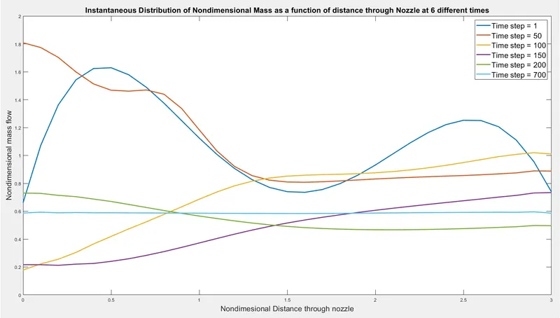
Figure 1. The mass Flow rate through the nozzle at different time step

The graph created from the program resembles graph 7.11 in Chapter 7 of John.D.Anderson book Computational Fluid Dynamics. In the above graph, the mass flow rate is varying through the nozzle during the initial time steps and becomes constant at time step equal to 700. At this time step, it can be said that the flow has achieved steady state.

Graph 2: Flowfield variables through the Nozzle distance with nozzle profile

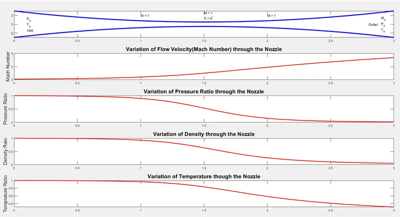
Figure 2. Flowfield variables through the Nozzle distance with nozzle profile

In the above graphs, the velocity of the flow increases through the nozzle and reaches a maximum velocity of 3.35 times the speed of sound. The velocity of the flow is equal to the speed of sound at the throat i.e Mach number = 1. As velocity increases the pressure, the density and temperature also decrease.

Graph 3: Timewise variation of the Flowfield variables at the nozzle throat

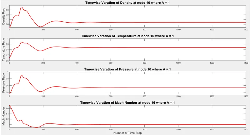
Figure 3. Timewise variation of the Flowfield variables at the nozzle throat

In the above graphs, all the flowfield variables in the non-dimensional form are unstable in the beginning and attain stability after 600 timesteps. This is due to the 'rubber band effect', i.e at early times the rubber band is stretched tightly and the flow field variables are driven by a stronger potential and hence change rapidly. At later times, as the steady-state is approached, the rubber band is less stretched and it becomes relaxed, and the changes become much smaller with time.

Conservation Form:

The program ran successfully and gave 3 Figures as output. In the first figure, the Mass Flow rate through the nozzle at different time step was plotted, in the second figure the Flowfield variables through the Nozzle distance with nozzle profile at the top are plotted and in the third figure, the Timewise variation of the Flowfield variables at the nozzle throat is plotted. The below graph shows the results of this program.

Graph 1: The mass Flow rate through the nozzle at different time step

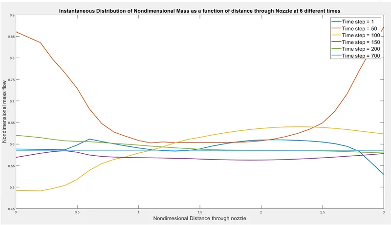
Figure 1. The mass Flow rate through the nozzle at different time step

The graph created from the program resembles graph 7.11 in Chapter 7 of John.D.Anderson book Computational Fluid Dynamics. In the above graph, the mass flow rate is varying through the nozzle during the initial time steps and becomes constant at time step equal to 700. At this time step, it can be said that the flow has achieved steady state.

Graph 2: Flowfield variables through the Nozzle distance with nozzle profile

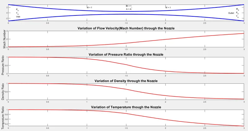
Figure 2. Flowfield variables through the Nozzle distance with nozzle profile

In the above graphs, the velocity of the flow increases through the nozzle and reaches a maximum velocity of 3.35 times the speed of sound. The velocity of the flow is equal to the speed of sound at the throat i.e Mach number = 1. As velocity increases the pressure, the density and temperature also decrease.

Graph 3: Timewise variation of the Flowfield variables at the nozzle throat

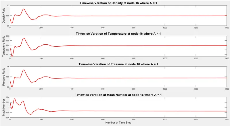
Figure 3. Timewise variation of the Flowfield variables at the nozzle throat

In the above graphs, all the flowfield variables in the non-dimensional form are unstable in the beginning and attain stability after 600 timesteps. This is due to the 'rubber band effect', i.e at early times the rubber band is stretched tightly and the flow field variables are driven by a stronger potential and hence change rapidly. At later times, as the steady-state is approached, the rubber band is less stretched and it becomes relaxed, and the changes become much smaller with time.

Graph 4: Comparison of Conservation and Nonconservation form of Governing equation for the Quasi 1-D Subsonic-Supersonic, Isentropic flow through Nozzle

After developing a separate program for conservation and non-conservation form, functions are created to calculate the solution for the conservation and non-conservation form and this function is used to plot the mass flow rate through the nozzle in the steady-state i.e at time step 1400.

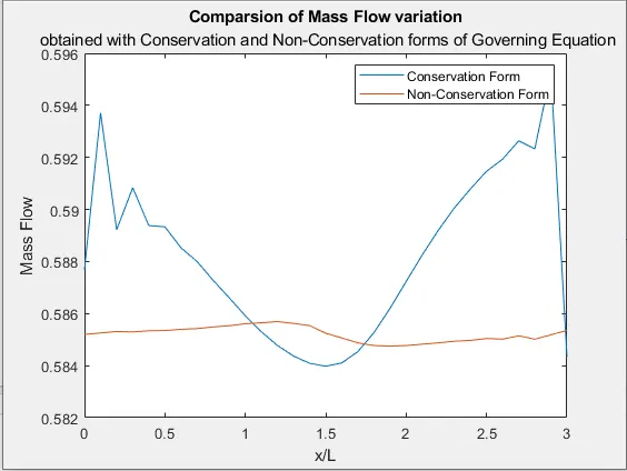
Figure 4: Comparison of Conservation and Nonconservation form of Governing equation for the Quasi 1-D Subsonic-Supersonic, Isentropic flow through Nozzle

The conservation form gives a distribution that is much closer to being a constant. In contrast, non-conservation results have( on the magnified scale) a sizeable variation, with some spurious oscillations at both the inflow and the outflow boundaries. On a practical basis, when plotted on the scale shown above, these variations are not apparent, and the mass flow essentially appears to be constant. The steady-state mass flow results obtained with the conservation form are much closer to the exact analytical solution.

Grid Dependancy:

Both the Conservation and Non-Conservation form of Governing equations to solve the Quasi 1-D Subsonic-Supersonic, Isentropic flow through Nozzle is ran for 61 grid points. The Stability of solution is mainly dependant on the Courant Number, and it should always less be than 1. In both the simulations, due to adaptive time step calculation at the end of each time step, the courant number is always constant and hence the program is grid independant.

CONCLUSION:

The program to simulate the isentropic flow through a quasi 1D subsonic-supersonic nozzle by deriving the conservation and non-conservation forms of the governing equations and solve them using MacCormack's technique. Also to determine the steady-state temperature distribution for the flow-field variables and investigate the difference between the two forms of governing equations by comparing their solutions is developed and results obtained are approximately matching the analytical solution.

From this project, it can be concluded that the conservation form does a better job of preserving mass throughout the flow field, mainly because the mass flow itself is one of the dependant variables in the equations-the mass flow is a primary result from these equations. In contrast, the dependant variables in the non-conservation form of teh equations are primitive variables, and the mass flow is obtained only as a secondary result.