Frontal Crash of the car BIW in RADIOSS

FRONTAL CRASH OF THE BIW IN RADIOSS

AIM: To conduct the simulation of frontal crash test of the given BIW of a car.

• Below image shows the image of the given BIW of the car.
• Check unit system and either follow[Mg mm s] or [Kg mm ms].
• Create appropriate interface ,friction 0.2 and recommended parameters.
• Make sure of no penetrations and intersection.
• Correct rigid bodies if any issues.
• Create rigid wall with friction 0.1.
• Compare the model weight with the full scale 300k nodes model and use added masses to reach target weight 700kg while getting CG about the required range.
• Initial velocity 35 mph.
• Use model checker to ensure good quality.
• Time-step :0.5 to 0.1 microseconds.
• Run 80 ms.

Output requests:

• Sectional force in the rails at location of indicated node 174247.
• Axial force received on the rails from bumper.
• Shotgun cross sectional forces.
• A pillar cross section.
• Acceleration curve received on the accelerometer at base of B pillar (on B pillar rocker).
• Intrusions on the dash wall 66695,66244.

Note:

1. Submit your simulation files including time and h3d files.
2. Plot energies and notice any difference.
3. Explain your errors and how to rectify?

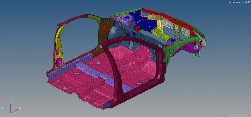
Image 1. BIW

INTRODUCTION

1. BIW(Body in White)

• Body-in-white is the name given to a car body's sheet when all its components have been welded together.
• BIW consists of barring moving parts (e.g., hoods, fenders, etc.), trims (e.g., glass, seats, etc.), or chassis sub assemblies.
• Image BIW shows the example of the BIW of a car.
• BiW constitutes about 27% of a car’s curb weight and remains the key determinant of how the car will perform.
• BiW can be made into two structures types.
• The more common monocoque structure where all body members are carrying load with chassis in-built with BiW and are integrated with each other.
• And the body-on-frame structure where the frame is the main load-carrying member.

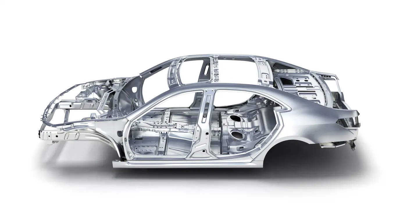
Image BIW

2. CRASH TEST

• A crash test is a form of destructive test usually performed in order to ensure safe design standards in crashworthiness and crash compatibility for various modes of transportation.
• Crash tests are conducted under rigorous scientific and safety standards.
• The main aim of these crash tests is to collect the data o how the car is crashed in actual accidents and impact on driver and passenger.
• There are many companies which conducts these physical car crash test to collect those data.
• Each crash test is very expensive, as complete vehicle is crashed, so the maximum amount of data must be extracted from each test.
• Usually, this requires the use of high-speed data-acquisition, at least one triaxial accelerometer and a crash test dummy, but often includes more.
• There are many types of crash tests, most common types of crash tests are

1. Frontal Impact test

2. Side Impact test

3. Roof Stremgth test

• For this project the Frontal Crash test is conducted on the BIW of car model.
• This model consist only front and middle section of the complete BIW of that car due to the limitation of the number of elements in the model to run the simulation.
• The maximum limit of number of nodes for the Student version of the Hypermesh is 1,00,000 nodes.
• The complete car model has more than 3,00,000 nodes which is not supported in the Student version of Hypermesh.
• Hence the frontal crash is made on the BIW and all the components are recreated using rigid bodies so as to reduce the number nodes.

3. FRONTAL CRASH TEST

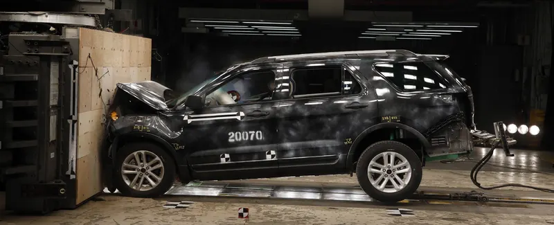
Image 3.1 Frontal Complete Crash Test

• Frontal car crash test is a type of Crash test by making the car to hit a solid concrete wall conducted
• This test is conducted to determine

1. Distribution of impact force on the BIW structure

2. Intrusion of the dashboard into the driver's cabin

3. Adult Occupant protection.

4. Child Occupant protection.

• The frontal crash is the most common cases of accidents i.e in most of the accidents involves frontal crash.
• There are four types of the frontal car crash

1. Moderate Overlap Frontal Crash test

2. Driver Side Small Overlap Frontal Crash test

3. Passenger Side Small Overlap Frontal Crash test.

4. Complete Frontal Crash test

• In this project Simulation of Complete Frontal Car Crash Rest is done on the given BIW of the car.
• For this project Only the distribution of forces and intrusion of the dashboard is calculated as there is no dummies present in the model.

PROCEDURE

1. Checking the unit system

• To check the unit system the radioss file is opened in the notepad
• Below the begin card there will be the unit system
• In this model the unit system was kg mm ms (refer the image 1.1.1)

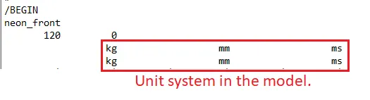
Image 1.1.1 Unit system in the model.

2. Checking for penetration

• Penetration is checked in the hypercrash as it is easier to find penetration in hypercrash than in hypermesh
• To check for penetration first model is imported in the hypercrash.
• To import the model drag the frontal_crash_0000.rad file from the file location and drop into the hypercrash window.
• To check for penetration Quality>Check All Solver Contact Interfaces.(refer the image 2.2)

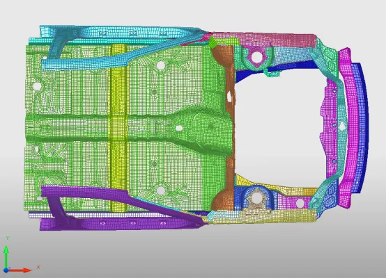
Image 2.1 Model

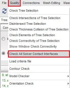
Image 2.2 Check penetration

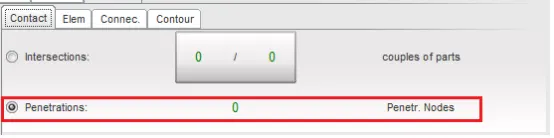
Image 2.3 No penetration

• In this model there was no penetrations.

3. Compare the model weight with the full scale 300k nodes model and use added masses to reach target weight 700kg while getting CG about the required range.

• To check for COG in the model Mass>Balancing
• A new will be opened below in that tab shows the total mass of the component and the location of the COG.
• Here the total mass of the component is shown in the tab.
• The total mass was found to be 188.42kg(refer the image 3.1)
• To check the COG location in the model click on the Show COG point icon(refer the image 3.2)

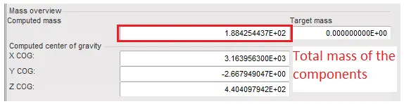
Image 3.1 Total mass of the car model before adding the mass.

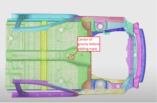
Image 3.2 COG initially

• The COG of the component is to be shifted rear of the initial position and the total mass of the components should be 700kg
• Total mass is to be 700kg because in the simulation only part of the car is involved. So by adding some mass at certain places will recreate those situation for example adding the mass of driver and his seat at the location of the seat mount in the floor panel.
• In this case mass is added at certain places, below table shows the how much mass is added for certain reason and its location.

Mass in kg	Description	Location
65	Driver and his seat	Floor Panel Image 3.2
65	Passenger and his seat	Floor Panel Image 3.3
170	Rear seat, spare wheel and fuel tank	Floor Panel Image 3.4
170	Rear seat, spare wheel and fuel tank	Floor Panel Image 3.5
42.1	Auxiliaries	Seat Reinforcement Image 3.6

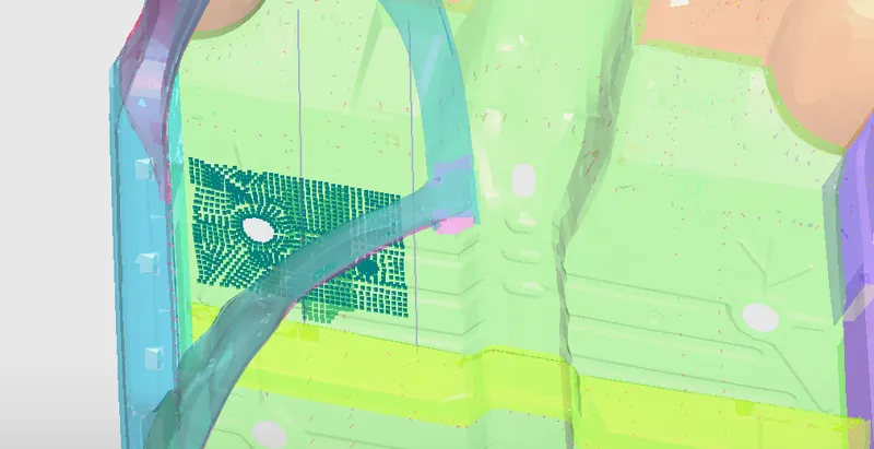
Image 3.2 65kg mass recreating the driver and his seat.

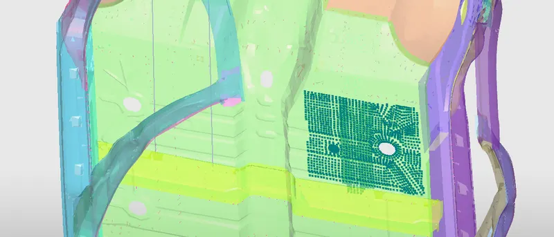
Image 1.3.3 65kg mass recreating the co-driver and his seat.

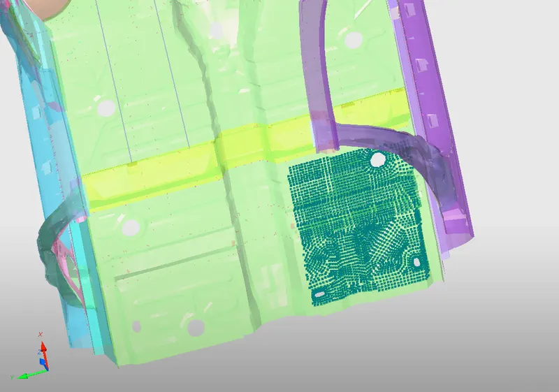
Image 3.4 170kg mass recreating the Rear seat, spare wheel and fuel tank.

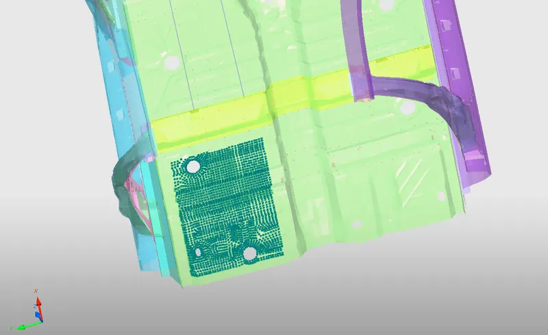
Image 3.5 170kg mass recreating the rear seat, spare wheel and fuel tank.

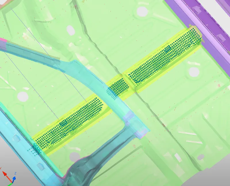
Image 3.6 42.1kg mass recreating the Auxiliaries.

• By adding these masses the total mass of the model was 700.5kg(refer the image 3.7)
• And the Center of Gravity was shifted rearwards and was below the Seat Reinforcement.(refer the image 3.8)

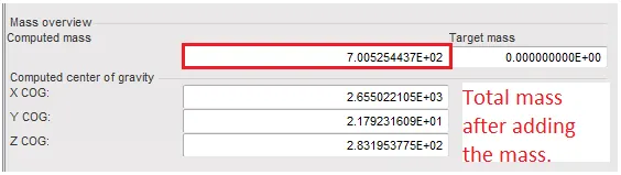
Image 3.7 Total mass of the model.

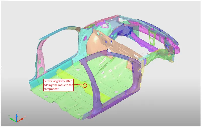
Image 3.8 Center of Gravity of the model.

4. Initial velocity of the model 35Mph

• For this crash test initial velocity is given to the model to recreate the crashing scenario.
• In this simulation the initial velocity given to the model is 35Mph or 15.6464mm/ms.
• To set the initial velocity of the model LoadCase>Initial Velocity>Set the value of the velocity in X-Direction>Select all nodes>Yes>Save.(refer the image 4.1)

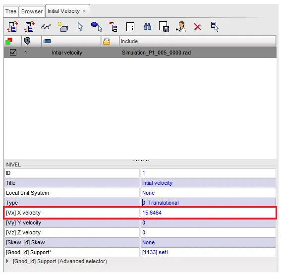
Image 4.1 Initial velocity

5. Time Step: 0.5 to 0.1 micro sec

• For this simulation the time step given is should be in between 0.5 micro sec to 0.1 micro sec.
• The time step selected for this simulation is 0.1micro sec I.e 0.0001ms which is the unit given in the simulation.
• Time step can be set in both in HyperCrash and in Hypermesh.
• This process is done in Hypermesh.
• To import the model in the Hypermesh Import>Solver Deck>Select the starter rad file>Import.(refer the image 5.1)

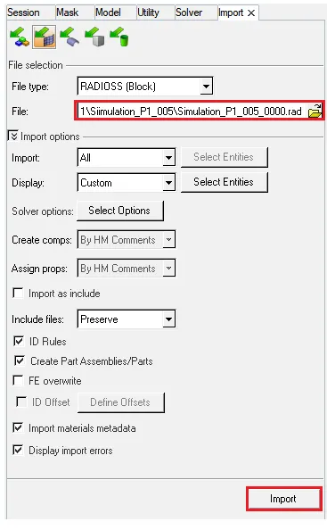
Image 5.1 Importing the model.

• To set the time step value Engine card should be created I.e DT card.
• To create this DT card Solver view> Create>Engine Keywords>DT>DT.(refer the image 5.2)
• In the DT card set the value of Tmin(time step) to 0.0001ms and Tscale as 0.9 (default vaue).(refer the image 5.3)

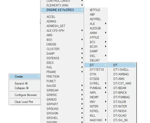
Image 5.2 DT.

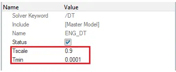
Image 5.3 DT card.

6. Run for 80ms.

• The run time for this simulation is 80ms I.e simulation of the frontal crash of the car is done for only 80ms.
• To set the value of the Run time to 80ms create ENG_RUN card.
• This card is created in the solver panel.
• To create ENG_RUN card Solver View>Create>Engine Keyword>Run.(refer the image 6.1)
• After creating the card set the value of Tstop to 80ms.(refer the image 6.2)

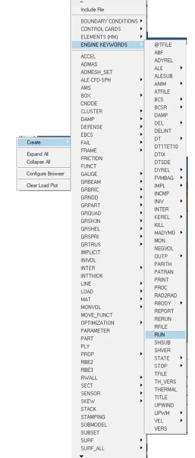
Image 6.1 ENG_RUN card

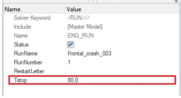
Image 6.2 Setting the value of Run time.

7. Output requests for the simulation.

7.1 Sectional force at the certain section of the car body.

• In the simulation section forces are calculated to check the distribution of forces of impact.
• The impact force is transferred from the bumper, which is the primary contact with the rigid wall, to the floor panel.
• To calculate the forces transferred through the components such as bumper to rails, through rails, through shotgun if the car and in A-Pillar a section is to be created on those components to view the forces.
• TO create a Section a frame of reference is needed, to create a frame Solver view>Create>FRAME>MOV> Now select the Origin Node, z axis and y-z plane node(refer the image 7.1.1).
• After creating the frame Solver View>Create>SECT>SECT> In the tab below Select the N1, N2 and N3 node for creating the skew> Select the frame>Select the group shell elements which are surrounding to the section>Set the value of Deltat and alpha as 0.1 and 0.67. (refer the Image 7.1.2)
• To check the section Model view>Cross Section>A-Pillar>Right click on A-pillar>Review>In the graphic area view the section if all the elements are inter connected.(refer the image 7.1.3)
• Similarly sections at other places are created.(refer the image 7.1.4)

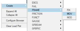
Image 7.1.1 Creating the frame

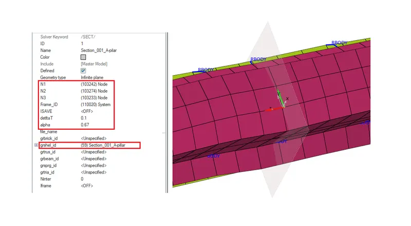
Image 7.1.2 Creation of Section

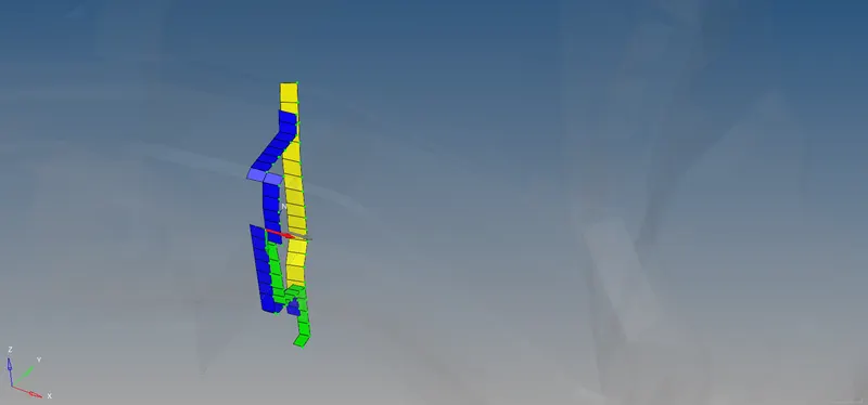
Image 7.1.4 Review of the Section created.

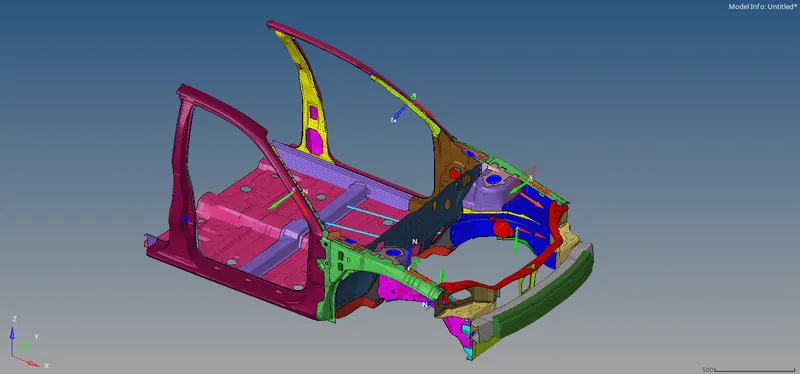
Image 7.1.4 All sections created at different location on the model.

7.2 Acceleration curve received on the accelerometer at base of B pillar (on B pillar rocker).

• Acceleration Curve is to be plotted inorder to find the deceleration of the car during the crash.
• To find the acceleration an accelerometer is to be placed on any node on the car component.
• To create a Accelerometer Solver View>Create>ACCEL>In the tab below Select the node ID>Select the node below the B-pillar on the Rocker in the model.(refer the image 7.2.1)
• Two accelerometer were created below the below the B-pillar of the car.

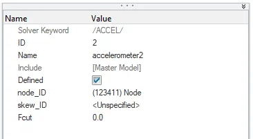
Image 7.2.1 Accelerometer.

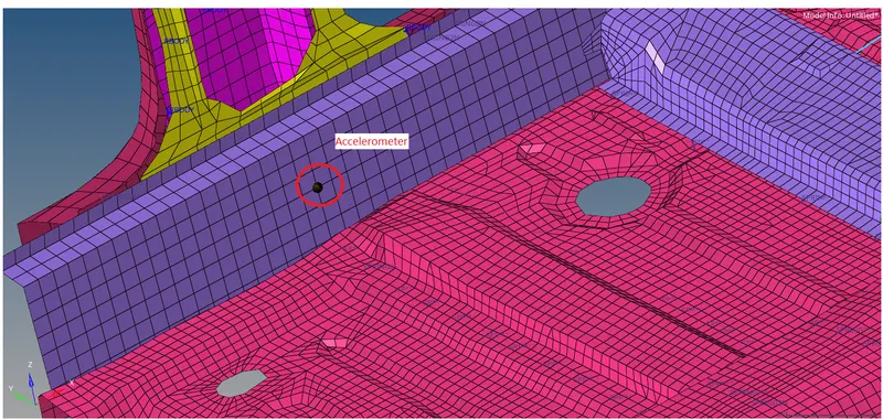
Image 7.2.2 Accelerometer location.

7.3 Intrusion on the Dash wall

• During the frontal crash of the car the passenger compartment tend to compress from the front i.e the floor panel tend to warp and compress the passenger compartment.
• Hence finding the displacement of the node at front end of the passenger compartment during the simulation will help in finding the percentage of compression of passenger compartment.
• Therefore to find the displacement a spring, with low stiffness and mass which will not vary the results, is created from front of the passenger compartment and a stationary point in the floor panel i.e cross member of the floor panel.
• To create a spring 1-D>Springs>Select the two nodes one at the font end of the passenger cabin and one at cross member.(refer the image 7.3.1)
• After creating the spring elements a property is assigned to that spring(refer the image 7.3.2).
• To find the compression of the spring a time history file is created.
• To create the TH file Solver view>Create>TH>SPRING>In the tab below select the two elements.(refer the image 7.3.3)

Image 7.3.1 Creating the Spring.

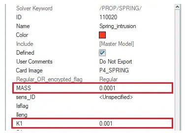
Image 7.3.2 Assigning the Property

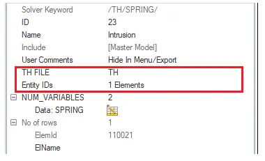
Image 7.3.3 Time history file for Spring Element.

8. Starting the Simulation of Frontal Crash of the given BIW

• To start the simulation Analysis>Radioss>Save as Name_0000.rad ina new folder>-nt 4 in the options for faster simulation>Radioss.(refer the image 8.1)

Image 8.1 Radioss

• Before running the file check for any errors in the model.
• To check the errors in the Hypermesh Tools>Model Checker>Radioss block(refer the image 8.1).
• Errors in the model is shown if there are any errors, also it will show the warnings.
• The solver will run the simulation if there are any warnings but will not if there are errors.
• To start the simulation Analysis>Radioss>Save as Name_0000.rad ina new folder>-nt 4 in the options for faster simulation>Radioss.(refer the image 8.3)

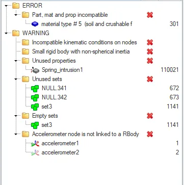
Image 8.1 Model Checker

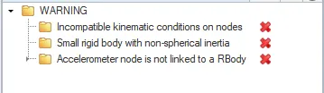
Image 8.2 Model Checker after clearing the errors

Image 8.3 Radioss

• On clicking the Radioss a new solver Screen will open, in that Solver screen all the calculation processe are shown.
• After completion of the simulation results button is shown in the solver screen.
• If there are errors in the model the Simulation will not run i.e in Solver screen it is shown as SOLVER FAILED.
• In the output file all the errors are shown with its ID.

RESULTS:

• This simulation took hrs to run completely and ran with NORMAL TERMINATION.
• The energy error of the simulation was found to be -2.2% which is in the accecptable range.
• Also the mass error was found to be 0.000 kg which is less than 1% of the total mass of the BIW.
• On clicking the Results button the animation of the simulation was shown in Hyperview.
• Animation 1.1 shows the animation of the Car BIW hitting the wall at 15.6464m/s speed.
• Using the Contour plot tool in the hyperview Von Mises stress induced in the BIW is shown.
• Animation 1.2 shows the Von Mises stress induced in the BIW during the test.

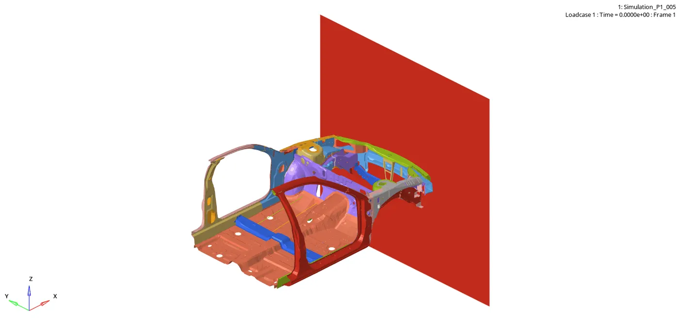
Animation 1.1 Simulation of the frontal crash.

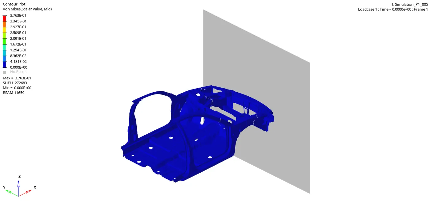
Animation 1.2 Von Mises stress induced in the car BIW.

GRAPHS:

1. GRAPH OF ENERGIES VS TIME GRAPH

• In the Hypergraph 2-D the graph of Energies vs Time is ploted.
• To plot the graph of the Energies vs Time Build Plots>Upload the Time history file>Select the X-Type to Time>Y-Type to Gobal variable>Y-Request- Contact Energy, Internal Energy, Kinetic Energy, Total energy and Hourglass energy>Y-Component MAG.(refer the image 1.1)
• Graph G.1 shows the graph of the Energies vs time.

Image 1.1 Build Plots.

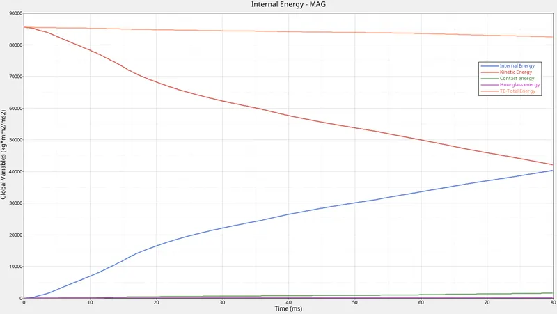
Graph G.1 Energies Vs Time.

• In the graph the Total energy of the simulation is decreases gradually as the contact energy increases.
• The maximum Contact energy of the simulation is 1.627991e+03 J.
• As the the BIW hits the rigid wall the Kinetic energy of the BIW reduces as the velocity is reduced.
• This Kintic energy is converted into deformation and hence the internal energy of the BIW is increasing.
• Since the simulation time only 80ms the velocity of the BIW does not reach zero.

Energies	Maximum Point	Minimum Point
Total Energy	8.560501e+04 J	8.251452e+04 J
Kinetic Energy	8.560501e+04 J	4.212489e+04 J
Internal Energy	4.038963e+04 J	0.000000e+00 J
Contact Energy	1.627991e+03 J	0.000000e+00 J
Hourglass Energy	2.227100e+02 J	0.000000e+00 J

2. GRAPH OF SECTION FORECS VS TIME

2.1 Section A-Pillar Left

• To plot the graph of Section forces vs Time Build Plots> Upload the Time history file>Select the X-Type to Time>Y-Type to Section Forces>Y-Request- Section_001_A-Pillar >Y-Component Resultant Normal Force, Resultant Tangent Forces and Resultant Total Force.(refer the image 2.1)
• Graph G.2 shows the graph of the Section vs time.

Image 2.1 Build Plots

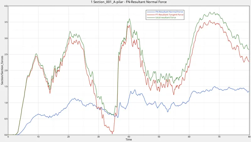
Graph G.2.1 Graph of Section Forces at A-Pillar vs time.

• From the graph the Total resultant force is increasing and decreasing 4 times as the deformation of the different section occur at different time of crash.
• Hence there is drop in the transfer of forces as this force is used in deforming the other BIW component.
• The Maximum force transfer through this A-Pillar section is 3.808517e+00 kN.

2.2 Section A-Pillar Right

• To plot the graph of Section forces vs Time Build Plots> Upload the Time history file>Select the X-Type to Time>Y-Type to Section Forces>Y-Request- Section_005_A-Pillar >Y-Component Resultant Normal Force, Resultant Tangent Forces and Resultant Total Force.
• Graph G.2.1 shows the graph of the Section vs time.

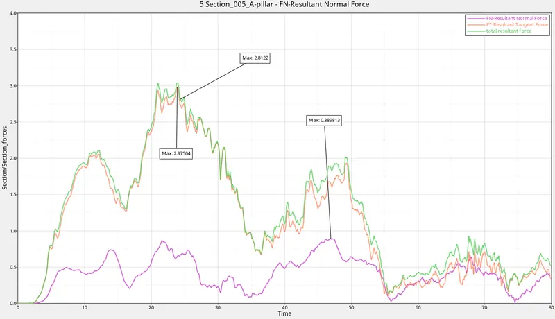
Graph G.2.2 Graph of Section Forces at A-Pillar vs time.

• From the graph the Total resultant force is increasing and decreasing 4 times as the deformation of the different section occur at different time of crash.
• Hence there is drop in the transfer of forces as this force is used in deforming the other BIW component.
• The Maximum force transfer through this A-Pillar section is 3.045166e+00 kN.

2.3 Section Shotgun Left

• To plot the graph of Section forces vs Time Build Plots> Upload the Time history file>Select the X-Type to Time>Y-Type to Section Forces>Y-Request- Section_003_Shotgun >Y-Component Resultant Normal Force, Resultant Tangent Forces and Resultant Total Force.
• Graph G.2.3 shows the graph of the Section vs time.

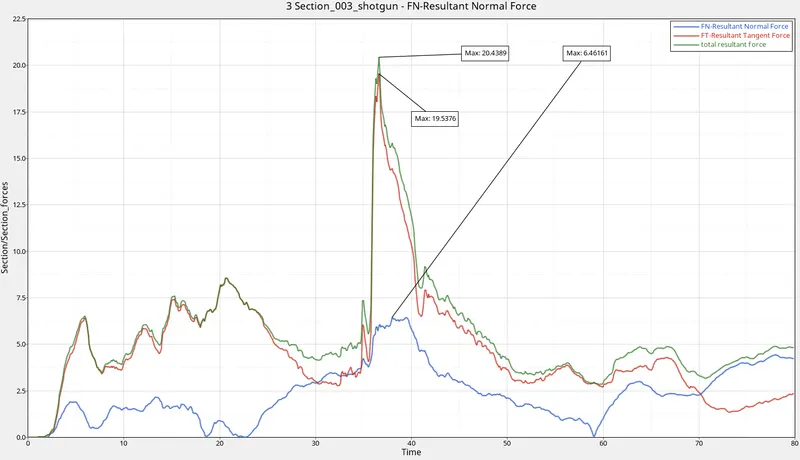
Graph G.2.3 Graph of the Section vs time.

• In this graph the forces transfer at the inital stages of crash is low and a sudden spike after 35ms.
• This spike is due the impact force on the shotgun as it hits the rigid wall.
• The Maximum force transfer through this Left Shotgun section is 2.043888e+01 kN.

2.4 Section Shotgun Right

• To plot the graph of Section forces vs Time Build Plots> Upload the Time history file>Select the X-Type to Time>Y-Type to Section Forces>Y-Request- Section_004_Shotgun >Y-Component Resultant Normal Force, Resultant Tangent Forces and Resultant Total Force.
• Graph G.2.4 shows the graph of the Section vs time.

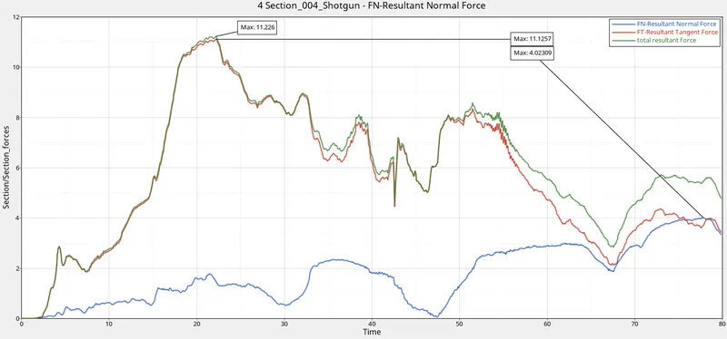
Graph G.2.4 Graph of the Section vs time.

• From the graph the resultant forces increases in the begining and decreases gradually.
• The Maximum force transfer through this Right Shotgun section is 1.122597e+01 kN.

2.5 Section Rails Right

• To plot the graph of Section forces vs Time Build Plots> Upload the Time history file>Select the X-Type to Time>Y-Type to Section Forces>Y-Request- Section_002_rail >Y-Component Resultant Normal Force, Resultant Tangent Forces and Resultant Total Force.
• Graph G.2.5 shows the graph of the Section vs time.

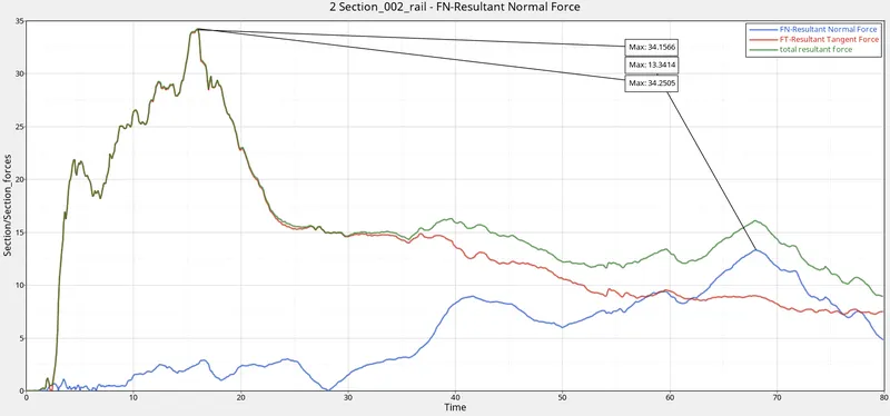
Graph G.2.5 Graph of the Section vs time.

• Most of the impact force is transfered to the car floor panel through this front rail.
• Since this rail transfers and absorbs most of the impact forces the maximum forces on the rail is 3.425047e+01 kN.
• These rails and the shotguns are the part of the crumble zone and hence should absorb most of the impact energy.

2.6 Section Rails Left

• To plot the graph of Section forces vs Time Build Plots> Upload the Time history file>Select the X-Type to Time>Y-Type to Section Forces>Y-Request- Section_006_rail >Y-Component Resultant Normal Force, Resultant Tangent Forces and Resultant Total Force.
• Graph G.2.6 shows the graph of the Section vs time.

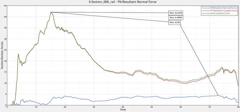
Graph G.2.6 Graph of the Section vs time.

• The Maximum force transfer through this Left Rail section is 4.207995e+01 kN.

3. GRAPH OF AXIAL FORCES TRANSFERED FROM BUMPER TO THE FRONT RAILS.

3.1 Right Bumper

• The force transfered from the bumper to the rails is known by creating a interface at bumper and the rail.
• To plot the graph of the interface forces vs time Build Plots> Upload the Time history file>Select the X-Type to Time>Y-Type to Interface/contact forces>Y-Request- 2 Right Bumper>Y-Component Resultant Normal Force, Resultant Tangent Forces and Resultant Total Force.

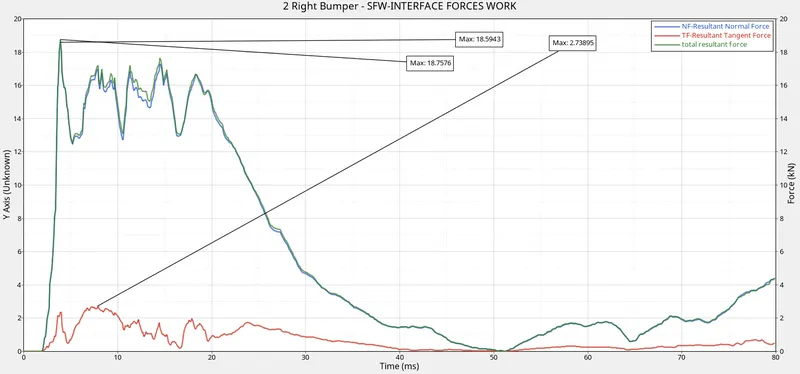
Graph G.3.1 Graph of the Interface forces vs time.

• From the graph the resultant forces increases suddenly in the begining and decreases gradually.
• The Maximum force transfer through this Right Shotgun section is 1.875761e+01 kN.

3.2 Left Bumper

• The force transfered from the bumper to the rails is known by creating a interface at bumper and the rail.
• To plot the graph of the interface forces vs time Build Plots> Upload the Time history file>Select the X-Type to Time>Y-Type to Interface/contact forces>Y-Request- 3 Left Bumper>Y-Component Resultant Normal Force, Resultant Tangent Forces and Resultant Total Force.

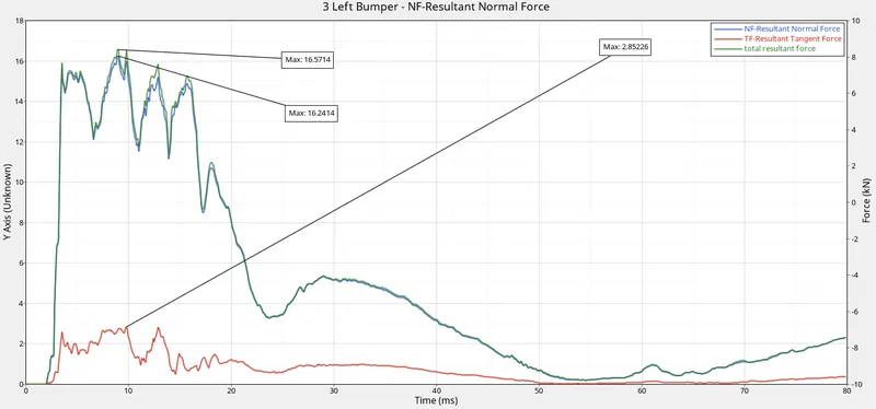
Graph G.3.2 Graph of the Interface forces vs time.

• From the graph the resultant forces increases suddenly in the begining and decreases gradually.
• The Maximum force transfer through this Right Shotgun section is 1.657143e+01 kN.

4. GRAPH OF ACCELERATION CURVE AT B-PILLAR.

• The deceleration of the car during the crash is very high, this high deceleration can risk the lives of the passengers of the vehicle.
• If the high impact energy is absorbed in the form of deformation at the front part of the car the deceleration of the passengers compartment will be less.
• Hence the frontal part of the car should be designed in such a way that it absorbs the most of the impact energy.
• Hence decelereation of the car during a crash is is to be determined to find the forces acing on the driver.
• To plot the graph of Deceleration at B-Pillar from an acclererometer is placed near the B-Pillar Build Plots> Upload the Time history file>Select the X-Type to Time>Y-Type to Accelerometer/Acceleration>Y-Request- 1 accelerometer >Y-Component ACC Resultant Acclereation.(refer the image 4.1)

Image 4.1 Build Plots

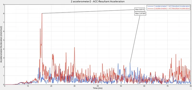
Graph G.4.1 Acceleration curve

• The maximum deceleration of the Left B-Pillar was found to be 8.011497e+00 mm/ms2 and at Left B-Pillar was 2.413455e+00 mm/ms2.

5. INTRUSION AT THE DASHBOARD

• To find the intrusion of the dashboard elongation of the spring of negligible mass and stiffness is deterimined.
• To plot the elongation of the spring Build Plots> Upload the Time history file>Select the X-Type to Time>Y-Type toSpring Elongation>Y-Request-110021>Y-Component Total elongation.(refer the image 5.1).

Image 5.1 Build Plots

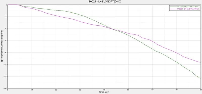
Graph G.5.1 Elongation of the Spring

• From the Graph the elongation is in Negative direction this is due to the compression of spring as the frontal part of the car is getting crushed.
• The maximum compression of the Brake pedal section i.e 66244 node was found to be 9.658583e+01 mm and that of Throttle Pedal i.e 66695 node was found to be 1.233512e+02 mm.

CONCLUSION:

The Frontal Crash Test of the given car BIW is Simluated in Hypermesh and required output requests are ploted and explained.

From the simulation Section forces at different location is shown using the Forces vs Time graph and deceleration of the car is determined using the Accelerometer placed at the B-Pillar.

Also the intrusion of the dashboard was found using the spring of negligible mass and stiffness.