Rankine cycle Simulator in MATLAB

Rankine Cycle Simulator

AIM: To create a Rankine Cycle Simulator using MATLAB

• Also to write a code should calculate the state points of the Rankine Cycle based on the User input.
• to plot the corresponding T-s and h-s plots for the given set of input with Titles and Labels.

THEORY: Rankine Cycle

• It is a model used to predict the performance of steam turbine systems.
• It was also used to study the performance of reciprocating steam engines.
• The Rankine cycle is an idealized Thermodynamic Cycle of a Heat Engine that converts heat into mechanical work while undergoing phase change.
• It is an idealized cycle in which friction losses in each of the four components are neglected. The heat is supplied externally to a closed loop, which usually uses water as the Working Fluid.
• This was developed by a Scottish Engineer, Willam J.M Rankine in 1859.
• Hence the name Rankline Cycle.

Processes in Rankine Cycle

There are four cycles in the Rankine Cycle. Below image shows the Physical Layout of the Rankine Cycle.

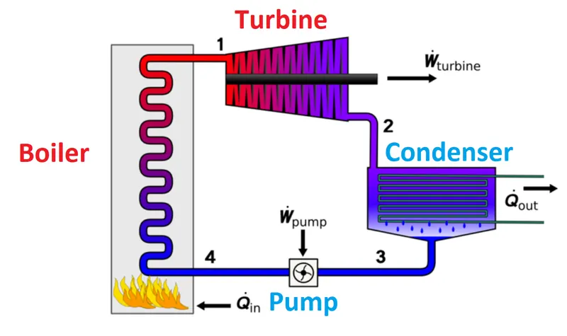
Image 1.1 Rankine Cycle layout.

• 1 - 2 Isentropic Compression: The working fluid is pumped from low pressure to High Pressure. As the fluid is at liquid state, the pump requires input energy.
• 2 - 3 Constant Pressure Heat Addition process: The high pressure liquid enters a boiler, where it is heated at constant pressure by an external heat source to become a dry vapour.
• 3 - 4 Isentropic Expansion: The Dry Saturated vapour expands through a turbine, generating power. This decreases the temperature and pressure of the vapour, and some condensation may occur.
• 4 - 1 Constant Pressure Heat rejection process: The wet vapour enters the condenser, where it is condensed at constant pressure to become saturated liquid.

The work input to the pump and the work output are calculated using enthalpy and entropy at that state using steam tables.

PROCEDURE:

Process Flow of the Rankine Cycle Simulator

1. Clearing all the data stored, closing all the figures and clearing the command window.
2. Displaying the name and description of the simulator.
3. Requesting for input by the user.
4. Calculating the standard values that are to be used in the program using the XSteam function.
5. Condition for working of the Rankine Cycle.
6. Calculating the parameters of the State points.
7. Calculating the Pump work required.
8. Calculating the heat input, heat rejected, thermal efficiency.
9. T-s curve calculation and plotting.
10. Enthalpy - Entropy curve calculation and plotting.
11. Displaying the result.

Step 1: Clearing all the data stored, closing all the figures and clearing the command window.

Below syntax is used to start the program with no previous data, figures.

clear all
close all
clc

• clear all - Clears the data stored in the work space.
• close all - Closes all the figures opened in the previous session.
• clc - Clears the command window.

Step 2: Displaying the name and description of the simulator.

The program should display the description of the cycle. Below syntax displays the following details about the cycle

RANKINE CYCLE SIMULATOR
1-2 is Isentropic Expansion in the Turbine
2-3 is Constant Pressure Heat rejection process
3-4 is Isentropic compression in the Pump
4-1 is Constant Pressure Heat addition process

disp('                                       RANKINE CYCLE SIMULATOR                                     ')
disp(' 1-2 is Isentropic Expansion in the Turbine')
disp(' 2-3 is Constant Pressure Heat rejection process')
disp(' 3-4 is Isentropic compression in the Pumpp')
disp(' 4-1 is Constant Pressure Heat addition process')

Step 3: Requesting for input by the user.

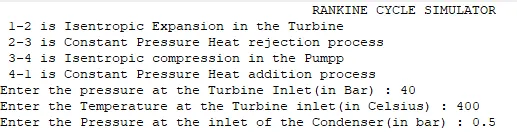
This program is developed in such a way that it calculate the state points based on the user inputs. Below syntax is used to collect the data i.e Inlet Temperature, Inlet Pressure at the turbine and Pressure at Turbine outlet.

p1 = input('Enter the pressure at the Turbine Inlet(in Bar) : ');
T1 = input('Enter the Temperature at the Turbine inlet(in Celsius) : ');
p2 = input('Enter the Pressure at the inlet of the Condenser(in bar) : ');

The above syntax displays text and receive the pressure and temperature inputs from the user. Below image shows how the data is stored in the respective location.

Step 4: Calculating the standard values that are to be used in the program using the XSteam function.

XSteam.m is a function which acts as Steam Tables that are used in solving the Rankine Cycle problem and other heat engine problems. Steam table is typically used to determine saturated steam temperature from steam pressure, or the opposite: pressure from saturated steam temperature. In addition to pressure and temperature, these tables usually include other related values such as specific enthalpy (h) and specific volume (v).

Standard values for this problem are

1. Saturation Vapour Entropy
2. Saturation Liquid Entropy
3. Saturation Vapour Enthalpy
4. Saturation liquid Enthalpy

Below syntax is used to calculate the standard values

sf1 = XSteam('sL_p',p1);            %Saturation Liquid Entropy for pressure at Turbine inlet
sg1 = XSteam('sV_p',p1);            %Saturation Vapour Entropy for pressure at Turbine inlet

sf2 = XSteam('sL_p',p2);            %Saturation Liquid Entropy for pressure at Turbine outlet
sg2 = XSteam('sV_p',p2);            %Saturation Vapour Entropy for pressure at Turbine outlet

hf2 = XSteam('hL_p',p2);            %Saturation Enthalpy for pressure at Turbine outlet
hg2 = XSteam('hV_p',p2);            %Saturation Vapour Enthalpy for pressure at Turbine outlet

Step 5: Condition for working of the Rankine Cycle.

The Rankine Cycle would work only when the inlet temperature at the turbine is more the Saturation Vapour Temperature at Inlet Pressure.

This condtion is adapted to the program by calculating the Saturation Vapour Temperature at inlet pressure.

Below if-else condition is used in the program.

if T1 <= Temp_03
    disp('The Cycle cannot have %f as Inlet Temperature',T1)

else

.
Rest of the program
.


end

Step 6: Calculating the parameters of the State points.

This cycle has four state points, to calculate the parameters at those state points XSteam.m is used.

For each state point following must be calculated

1. Entropy at that state
2. Enthalpy
3. Temperature
4. Pressure

1. State Point 1: At state point 1 i.e turbine inlet, entropy and enthalpy is calculated as the pressure and temperature are taken from user.

Below syntax is used to find the Specific entropy and enthalpy using the XSteam function for defined inlet pressure and temperature.

s1 = XSteam('s_pT',p1,T1);          %Entropy at the Turbine inlet
h1 = XSteam('h_pT',p1,T1);          %Enthalpy at the Turbine inlet

2. State Point 2: At state point 2, i.e condenser inlet, the entropy will be same as the entropy at state 1 as the process 1 - 2 is Isentropic. And the enthalpy is calculated by graphical method using the saturatioin vapour enthalpy and entropy and saturation liquid enthapy and entropy.

The enthalpy at the inlet of the condenser is shown below

`(sunderset(2)( )-sunderset(f2)( ))/(sunderset(g2)( ) -sunderset(f2)( )) =(hunderset(2)( ) - hunderset(f2)( ))/(hunderset(g2)( ) - hunderset(f2)( )`

Below code is used to calculate the enthalpy using the above equation

s2 = s1;                            %Specific Entropy at Turbine inlet = Specific Enrtropy at Turbine outlet(Isentropic Process)

x2 = (s2-sf2)/(sg2-sf2);            
h2 = hf2 + (x2*(hg2-hf2));          %Enthalpy at the Turbine outlet

The temperature at the inlet of the condenser is as same as the temperature at the outlet of the condenser which is the saturation temperature for pressure at the inlet of the condenser.

3. State Point 3: At state point 3, i.e at pump inlet, the pressure is as same as the state 3 as the process of condenser is Isobaric i.e constant pressure process.

Temperature at this state is Saturation temperature of water at pressure at pump inlet.

Below syntax is used to calculate the parameters of State point 3

%Inlet Pressure of the condenser = Inlet Pressure of Pump
p3 = p2;
h3 = XSteam('hL_p',p3);             %Enthalpy at Pump intlet
s3 = XSteam('sL_p',p3);             %Entropy at Pump intlet
T3 = XSteam('Tsat_p',p3);           %Temperature at the intlet of pump
T2 = T3;                            %Inlet Temperature of Condenser = Oulet Temperature of Condenser 
v3 = XSteam('vL_p',p3);             %Specific Volume

4. State Point 4: At state point 4, i.e at boiler inlet or pump outlet, pressure at this point is as same as the pressure turbine inlet, and entropy is as same as the entropy at previous state as the pump process is isentropic process.

Below syntax is used to calculate the temperature at the inlet of boiler as the pump heats the water during the pumping process which is calculated using the XSteam function as a function of entropy and pressure.

%Inlet Pressure of the Turbine = Outlet pressure of the pump
p4 = p1;
s4 = s3;                            %Entropy at Pump inlet = Entropy at Pump outlet
T4 = XSteam('T_ps',p4,s4);          %Outlet temperature of the Pump

Step 7: Calculating the Pump work required and Work done by Turbine

To calculate the Enthalpy at this state work done on the pump is to calculated.

Below equation is used to calculate the Work fone on the pump

`Wp=vunderset(3)( ) *(punderset(4)( )-punderset(3)( ))`

`Wp = dot m* (hunderset(4)( ) -hunderset(3)( ))`

where,

`v` = Specific volume

`dot m` = Mass flow rate (here it is taken as 1)

`h` = enthalpy

`p` = pressure.

Below syntax is used to calculate the work done on the pump in order to increase the water pressure from low pressure to high pressure and enthalpy using the Work done on the pump.

Wp = v3*(p4-p3)*100;                %Amount of work required for the pump

h4 = h3 + Wp;                       %Enthalpy at inlet of the Boiler

Work done by the turbine is given by the following equation.

`Wt = dot m* (hunderset(1)( ) -hunderset(2)( ))`

`Wunderset(t)( ) = hunderset(1)( )-hunderset(2)( )`

where,

`dot m` = Mass flow rate (here it is taken as 1)

`h` = enthalpy

The Net work output is given by the following equation

`Wunderset(text(net))( ) = Wunderset(t)( ) - Wunderset(p)( )`

By using the above equations the Output

%Work Output

Wt = h1-h2;                         %Work done by Turbine
Wnet = Wt-Wp;                       %Net Work

Step 8: Calculating the heat input, heat rejected, thermal efficiency.

Below equations are used to calculate the heat input, heat rejected and thermal efficiency.

Heat Input

`Qunderset(text(in))( ) = hunderset(1)( ) - hunderset(4`

Heat Rejected

`Qunderset(text(out))( ) = hunderset(2)( ) - hunderset(3`

Thermal Efficiency

`etaunderset(thermal)( ) = (Wunderset(text(net))( ) )/(Qunderset(text(in))`

% Heat Input
Qin = h1-h4;
%Heat Rejected in the condenser
Qout = h2-h3;

%Thermal Efficiency
ntherm = Wnet/Qin;

Step 9: T-s curve calculation and plotting.

Saturation Vapour and Saturation liquid curve for water

To plot this curve first the values are to be calculated

Below syntax is used to calculate the Saturation Temperature and entropy for the pressure ranging from 0 till 1000 bar.

Pressure = linspace(0,1000,6000);   %Pressure range for plotting the T-S curve for the Water using the XSteam function
for i = 1:length(Pressure)
    EntropyL(i) = XSteam('sL_p', Pressure(i));
    Temperature(i) = XSteam('Tsat_p', Pressure(i));
    EntropyV(i) = XSteam('sV_p',Pressure(i));
end

The above syntax will calculate the values of saturation vapour temperature and entropy and saturation liquid temperature and entropy.

These values are used to plot the T-s curve of Water.Below syntax is sued to plot the same.

plot(EntropyL,Temperature,'color','#4DBEEE','linewidth',2)
plot(EntropyV,Temperature,'color','#4DBEEE','linewidth',2)

In the Rankine cycle State 1-2, 2-3 and 3-4 is a straight line and the state 4-1 is curve.

To calculate the points for the 4-1 curve below syntax is used.

%Calculation for T-S Curve for Inlet Pressure  
e_1_p1 = linspace(sf2,sf1,100);
e_2_p1 = linspace(sg1,s1,100);
for i = 1:length(e_1_p1)
    Temp_01(i) = XSteam('T_ps',p1,e_1_p1(i));
    Temp_02(i) = XSteam('T_ps',p1,e_2_p1(i));
end

The above syntax calculates the temperatures(Temp_01) ranging from saturation liquid entropy for low pressure till saturation liquid entropy for high pressure and Temperatures(Temp_02) ranging from saturation vapour entropy for high pressure till saturation vapour entropy for low pressure of the system. The temperature is constant from the saturation liquid entropy till saturation vapour entropy for high pressure. The below syntax is used to plot the Rankine Cycle.

figure(1)
plot([s1 s2],[T1 T2],'color','#77AC30','linewidth',3)
hold on
title('T-S curve for Rankine Cycle')
xlabel('Entropy[J/C]')
ylabel('Temperature[C]')
text(s1,T1,'1')
text(s2,T2,'2')
text(s3,T3,'3')
text(s4,T4,'4')
plot([s2 s3],[T2 T3],'color','#77AC30','linewidth',3)
plot([s3 s3],[T3 T4],'color','#77AC30','linewidth',3)
plot(EntropyL,Temperature,'color','#4DBEEE','linewidth',2)
plot(EntropyV,Temperature,'color','#4DBEEE','linewidth',2)
plot(e_1_p1,Temp_01,'color','#77AC30', 'linewidth',3)
plot(e_2_p1,Temp_02,'color','#77AC30','linewidth',3)
plot([sf1 sg1],[Temp_03 Temp_03],'color','#77AC30','linewidth',3)

Step 10: Enthalpy - Entropy curve calculation and plotting.

The below syntax is used to calculate the enthalpy for pressure ranging from 0 to 1000 bar for h-s curve of water.

% Calculation for Enthalpy-Entropy graph
for i = 1:length(Pressure)
    EnthalpyL(i) = XSteam('hL_p', Pressure(i));
    EnthalpyV(i) = XSteam('hV_p',Pressure(i));
end

Below syntax is used to plot the h-s curve of water.

plot(EntropyL,EnthalpyL,'color','#4DBEEE','linewidth',1)

Since the variation of the enthalpy is linear only end points are required to plot the Rankine Cycle.

Below syntax is used to plot the h-s curve for Rankine cycle.

%Plotting the Enthalpy-Entropy graph
figure(2)
plot(EntropyL,EnthalpyL,'color','#4DBEEE','linewidth',1)
hold on
title('h-s curve for Rankine Cycle')
ylabel('Enthalpy [kJ/kg C]')
xlabel('Entropy[J/C]')
text(h1,T1,'1')
text(h2,T2,'2')
text(h3,T3,'3')
text(h4,T4,'4')
plot(EntropyV,EnthalpyV,'color','#4DBEEE','linewidth',1)
plot([s1 s2 s3 s4 s1],[h1 h2 h3 h4 h1],'color','#77AC30','linewidth',2)

This curve is to be plotted in another figure and hence figure(2) is used.

Step 11: Displaying the result.

After calculating and plotting the result, it should be displayed in teh command window. In the command window parameters for all the state points, work done, heat input and thermal efficiency are to be mentioned. The below syntax is used to display the results in command window.

Temperatures = [T1,T2,T3,T4];
Pressures = [p1,p2,p3,p4];
Entropies = [s1,s2,s3,s4];
Enthalpies = [h1,h2,h3,h4];

for i = 1:4
    
    sprintf('At State point %f',i);
    disp('P%f is : %f',i,Pressures(i));
    disp('T%f is : %f',i,Temperature(i));
    disp('H%f is : %f',i,Enthalpies(i));
    disp('S%f is : %f',i,Entropies(i));
    
end

The 'for' loop is used to display the results so as to simplify the code.

PROGRAM:

The complete program is shown below.

% Progrm to simulate the Rankine Cycle by taking the user inputs

%Clearing the data stored in the workspace, closing all the figure and
%clearing the command window
clear all
close all
clc

%Displaying the name of the simulator
disp('                                       RANKINE CYCLE SIMULATOR                                     ')
disp(' 1-2 is Isentropic Expansion in the Turbine')
disp(' 2-3 is Constant Pressure Heat rejection process')
disp(' 3-4 is Isentropic compression in the Pumpp')
disp(' 4-1 is Constant Pressure Heat addition process')

%Taking the input ffrom the user
p1 = input('Enter the pressure at the Turbine Inlet(in Bar) : ');
T1 = input('Enter the Temperature at the Turbine inlet(in Celsius) : ');
p2 = input('Enter the Pressure at the inlet of the Condenser(in bar) : ');


%%
%Properties of watercalculated from XSteam function

sf1 = XSteam('sL_p',p1);            %Saturation Liquid Entropy for pressure at Turbine inlet
sg1 = XSteam('sV_p',p1);            %Saturation Vapour Entropy for pressure at Turbine inlet

sf2 = XSteam('sL_p',p2);            %Saturation Liquid Entropy for pressure at Turbine outlet
sg2 = XSteam('sV_p',p2);            %Saturation Vapour Entropy for pressure at Turbine outlet

hf2 = XSteam('hL_p',p2);            %Saturation Enthalpy for pressure at Turbine outlet
hg2 = XSteam('hV_p',p2);            %Saturation Vapour Enthalpy for pressure at Turbine outlet


Temp_03 = XSteam('T_ps',p1,sf1);    % Saturation Temperature for the Inlet Pressure
%%
%Condition for Rankine Simulator to Run

if T1 <= Temp_03
    F = sprintf('The Cycle cannot have %f C as Inlet Temperature',T1);
    disp(F)

else
%%
%State Point 1

%Turbine Inlet Pressure- user input value

s1 = XSteam('s_pT',p1,T1);          %Entropy at the Turbine inlet
h1 = XSteam('h_pT',p1,T1);          %Enthalpy at the Turbine inlet


%% 
% State Point 2 Turbine outlet or Condenser inlet

s2 = s1;                            %Specific Entropy at Turbine inlet = Specific Enrtropy at Turbine outlet(Isentropic Process)

x2 = (s2-sf2)/(sg2-sf2);            
h2 = hf2 + (x2*(hg2-hf2));          %Enthalpy at the Turbine outlet


%%
% State Point 3 Condenser outlet or Pump inlet

%Inlet Pressure of the condenser = Inlet Pressure of Pump
p3 = p2;
h3 = XSteam('hL_p',p3);             %Enthalpy at Pump intlet
s3 = XSteam('sL_p',p3);             %Entropy at Pump intlet
T3 = XSteam('Tsat_p',p3);           %Temperature at the intlet of pump
T2 = T3;                            %Inlet Temperature of Condenser = Oulet Temperature of Condenser 
v3 = XSteam('vL_p',p3);             %Specific Volume

%%
%State Point 4

%Inlet Pressure of the Turbine = Outlet pressure of the pump
p4 = p1;
s4 = s3;                            %Entropy at Pump inlet = Entropy at Pump outlet
T4 = XSteam('T_ps',p4,s4);          %Outlet temperature of the Pump


% Pump Work
Wp = v3*(p4-p3)*100;                %Amount of work required for the pump

h4 = h3 + Wp;                       %Enthalpy at inlet of the Boiler

%%
%Work Output

Wt = h1-h2;                         %Work done by Turbine
Wnet = Wt-Wp;                       %Net Work

%% 
% Heat Input
Qin = h1-h4;
%Heat Rejected in the condenser
Qout = h2-h3;

%Thermal Efficiency
ntherm = Wnet/Qin;

%%
%Calculation for T-S curve for Water

Pressure = linspace(0,1000,6000);   %Pressure range for plotting the T-S curve for the Water using the XSteam function
for i = 1:length(Pressure)
    EntropyL(i) = XSteam('sL_p', Pressure(i));
    Temperature(i) = XSteam('Tsat_p', Pressure(i));
    EntropyV(i) = XSteam('sV_p',Pressure(i));
end

%%
%Calculation for T-S Curve for Inlet Pressure  
e_1_p1 = linspace(sf2,sf1,100);
e_2_p1 = linspace(sg1,s1,100);
for i = 1:length(e_1_p1)
    Temp_01(i) = XSteam('T_ps',p1,e_1_p1(i));
    Temp_02(i) = XSteam('T_ps',p1,e_2_p1(i));
end

%%
%Plotting the State points and the T-S curve of water
figure(1)
plot([s1 s2],[T1 T2],'color','#77AC30','linewidth',3)
hold on
title('T-S curve for Rankine Cycle')
xlabel('Entropy[J/C]')
ylabel('Temperature[C]')
plot([s2 s3],[T2 T3],'color','#77AC30','linewidth',3)
plot([s3 s3],[T3 T4],'color','#77AC30','linewidth',3)
plot(EntropyL,Temperature,'color','#4DBEEE','linewidth',2)
plot(EntropyV,Temperature,'color','#4DBEEE','linewidth',2)
plot(e_1_p1,Temp_01,'color','#77AC30', 'linewidth',3)
plot(e_2_p1,Temp_02,'color','#77AC30','linewidth',3)
plot([sf1 sg1],[Temp_03 Temp_03],'color','#77AC30','linewidth',3)

%%
% Calculation for Enthalpy-Entropy graph
for i = 1:length(Pressure)
    EnthalpyL(i) = XSteam('hL_p', Pressure(i));
    EnthalpyV(i) = XSteam('hV_p',Pressure(i));
end

%%
%Plotting the Enthalpy-Entropy graph
figure(2)
plot(EntropyL,EnthalpyL,'color','#4DBEEE','linewidth',1)
hold on
plot(EntropyV,EnthalpyV,'color','#4DBEEE','linewidth',1)
plot([s1 s2 s3 s4 s1],[h1 h2 h3 h4 h1],'color','#77AC30','linewidth',2)



%%
%Printing the Output

Temperatures = [T1,T2,T3,T4];
Pressures = [p1,p2,p3,p4];
Entropies = [s1,s2,s3,s4];
Enthalpies = [h1,h2,h3,h4];

disp('RESULTS')
for i = 1:4
    
    S = sprintf('nnn At State point %d',i);
    A = sprintf('P%d is : %f bar',i,Pressures(i));
    B = sprintf('T%d is : %f C',i,Temperatures(i));
    C = sprintf('H%d is : %f kJ/kg',i,Enthalpies(i));
    D = sprintf('S%d is : %f J/C ',i,Entropies(i));
    disp(S)
    disp(A)
    disp(B)
    disp(C)
    disp(D)
end
end

RESULTS:

On running this program, it requested for user input for Inlet Pressure, Inlet Temperature and Outlet pressure. After giving the inputs the program created a Rankine Cycle from the user inputs and plotted the T-s curve and h-s curve. Also the results are displayed in the command window.

Below images shows the T-s and h-s curve for the user inputs

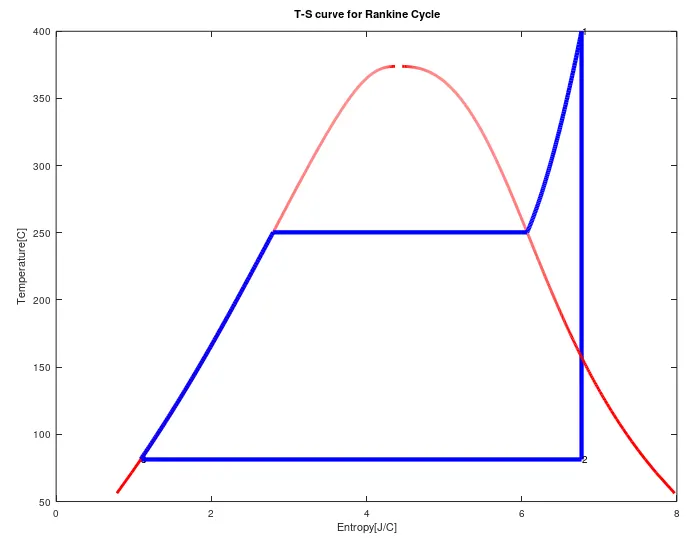
Graph 1. T-s Curve

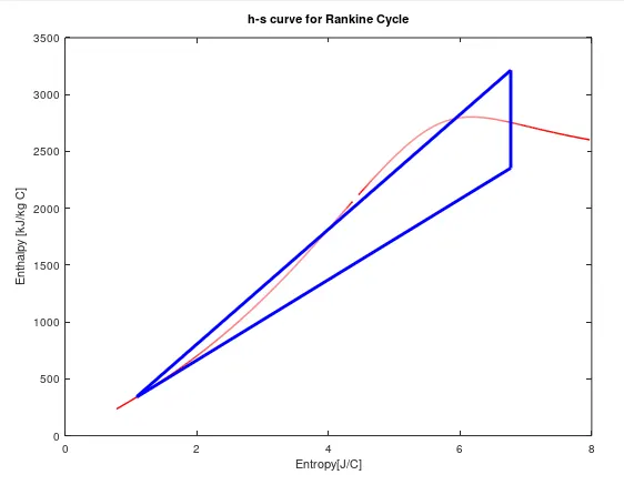
Graph 2. h-s Curve

CONCLUSION:

The program named Rankine Cycle Simulator which receives user inputs(inlet pressure, inlet temperature and outlet pressure) and displays the parameters of the Rankine Cycle and Plots the T-s and h-s curve. Also it has condition for working of Rankine Cycle it the condition is not satisfied it displays "The Rankine Cycle cannot have the Inlet Temperature that the user have given".