Week 7 - Simulation of a 1D Super-sonic nozzle flow simulation using Macormack Method
Objective :
Case : 1D Supersonic flow through a convergent-divergent nozzle.
a) To derive and solve conservative and non-conservatice forms of governing equations for and solve them using MacCormack's method .
b) Determine steady state temperature distribution for flow field variables and differentiate between two forms of governing equations by comparing their solutions .
c) Plot
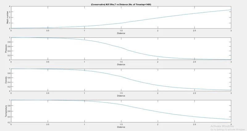
1. Steady-state distribution of primitive variables inside the nozzle
2. Time-wise variation of the primitive variables
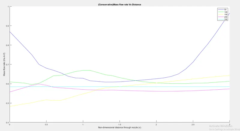
3. Variation of Mass flow rate distribution inside the nozzle at different time steps during the time-marching process
4. Comparison of Normalized mass flow rate distributions of both form
Theory :
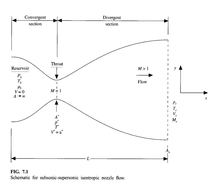
Consider an isentropic flow through a convergent-divergent nozzle with length L or x .
Inlet variables Variables at throat Variables at Exit
Pressure = `P_o` `P^*` `P_e`
Temperature = `T_o` `T^*` `T_e`
Velocity = `V_o` `V^*` `V_e`
Area= `A_o` `A^*` `A_e`
Mach number M<1 M=1 M>1
The area at the opening is very large , hence the velocity is considered to be very small (approximately 0) .
The velocity increases as it passes through the nozzle and exits at supersonic speed . The area is minimum at throat and here velocity is considered to be equal to speed of sound (M=1) . Here the sectional area varies as a function of distance x . Here we consider that the variables vary along x direction only . Hence we consider this as a quasi-one-dimensional flow . The pressure difference at inlet and outlet leads to the increase in velocity .
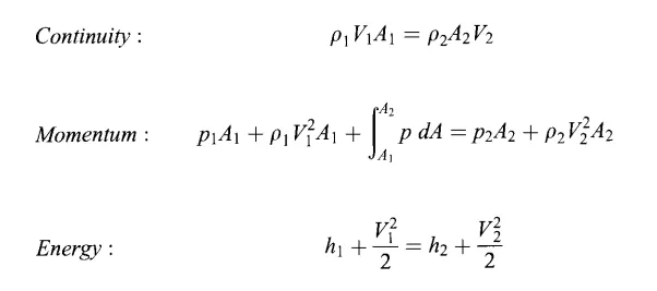
Given below are the governing equations for quasi-one -dimesional flow .
The mach number variation along the nozzle is exclusively governed by the below equation
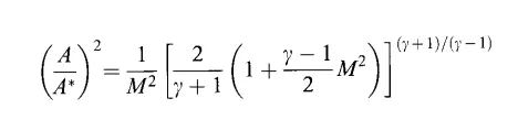
where `gamma=C_p/C_v=1.4` for standard conditions of air .
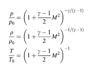
Similarly , equations for variation in pressure , density and temperature are given below .
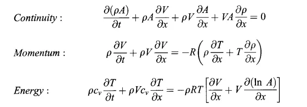
Since the quasi-one-dimensional assumption twists certain aspects of physics , we take the integral form of governing equations and work with them so that the physical aspects remain true . Hence we can re-write the governing equations in following manner .
Governing equations :
Governing equations in conservative form
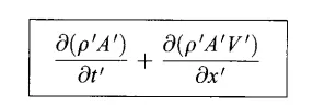
Continuity Equation
Momentum Equation

Energy Equation

Governing equations in non-conservative form
Continuity Equation

Momentum Equation

Energy Equation

Initial & Boundary Condition :
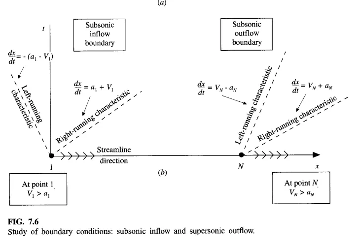
While looking at the diagram ,we can observe that the inlet and outlet variables depend on time rate of change of velocities .
Hence we use Von-Neumann boundary conditions .
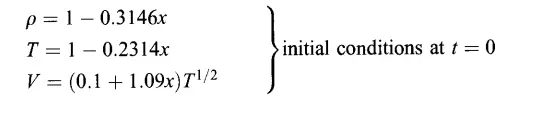
In non-conservative form, we consider the following initial and boundary conditions
initial condition
Boundary condition
at inlet

at oulet
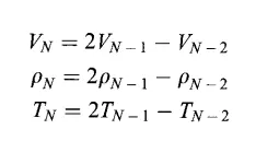
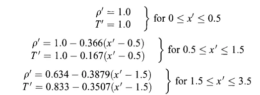
In conservative form , we use following initial conditions ,
boundary condition at inlet


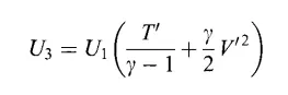
at outlet
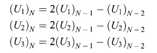
where N=i .
Discretization scheme used :
By MacCormack's Method ,
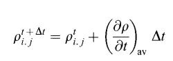
where `rho_(i,j)^(t+trianglet)` is the density at next time step
`rho_(i,j)^t` is the density at present time step .
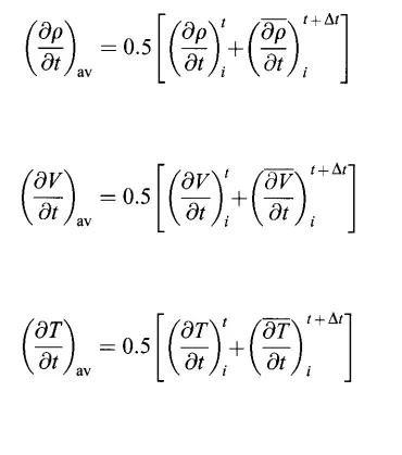
`((delrho)/(delt))_(av)` is the partial derivative of density obtained from predictor and corrector step .
`trianglet` is the time step .
Equations for predictor and corrector step are given below .
predictor step :
Equation for density by replacing partial differences with forward differences,
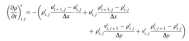
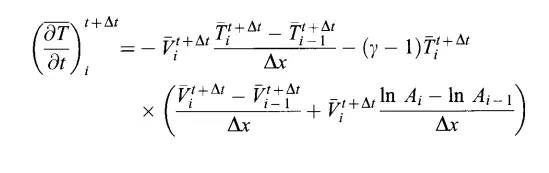
Using above method , we obtain equation for predicted density, velocity and temperature at next time step
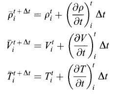
Corrector step
Equation for density by replacing partial derivatives with rearward differences ,
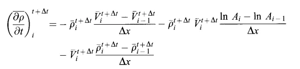
similarly we can apply for temperature and velocity as well .

Equation for average calculation .
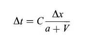
Equation for time step
Hence we can obtain solution for density , velocity and temperature by applying all the above values in first equation under MacCormacks method .
Main Code :
1) Main code
clear all
close all
clc

n=input('Enter number of grid points ');
x=linspace(0,3,n);
gamma=1.4;
dx=x(2)-x(1);


%area
 a=1+(2.2*(x-1.5).^2);

% timestep
nt=1400;


% Non -conservative
[rho,v,t,M,p,m,p_t,rho_t,t_t,M_t]=non_conservative(n,nt);

%Conservative
[rho_c,v_c,t_c,M_c,p_c,m_c,p_tc,rho_tc,t_tc,M_tc]= conservative(n,nt);


% Non -conservative

% To plot variables Vs distance
figure(1)
subplot (4,1,1)
plot(x,M)
title_text=sprintf('(Non- Conservative)Dimensionless M,P,Rho,T vs Distance (No. of Timestep=%d)',nt);
title(title_text)
xlabel('Distance')
ylabel('Mach number')
hold on

subplot(4,1,2)
plot(x,p)
xlabel('Distance')
ylabel('Pressure')
hold on

subplot(4,1,3)
plot(x,rho)
xlabel('Distance')
ylabel('Density')
 hold on

subplot(4,1,4)
plot(x,t)
xlabel('Distance')
ylabel('Temperature')
hold on

% To plot variables at time step
figure(2)
nt=1:1400 ;
subplot(4,1,1)
plot (nt,t_t)
 title_text=sprintf( '(Non- Conservative) T,Rho,M,p VS Time step at throat at %d Grid points ',n)
 title(title_text)
xlabel('Time step')
ylabel('Temperature')
hold on


subplot(4,1,2)
plot(nt,rho_t)
xlabel('Time Step')
ylabel('Density ')
hold on

subplot(4,1,3)
plot(nt,M_t)
xlabel('Time Step')
ylabel('Mach Number')
hold on

subplot(4,1,4)
plot(nt,p_t)
xlabel('Time Step')
ylabel('Pressure')
hold on


% Conservative
nt=1400 ;
figure(3)
subplot(4,1,1)
plot(x,M_c)
title_text=sprintf('(Conservative) M,P,Rho,T vs Distance (No. of Timestep=%d)',nt)
title(title_text)
xlabel('Distance')
ylabel('Mach number')
hold on

subplot(4,1,2)
plot(x,p_c)

xlabel('Distance')
ylabel('Pressure')
hold on

subplot(4,1,3)
plot(x,rho_c)
xlabel('Distance')
ylabel('Density')
hold on

subplot(4,1,4)
plot(x,t_c)

xlabel('Distance')
ylabel('Temperature')
hold on

figure(4)
nt=1:1400 ;
subplot(4,1,1)
plot (nt,t_tc)
title_text=sprintf( ' (Conservative ) T,Rho,M,P VS Time step at throat at %d Grid points',n)
title(title_text)
xlabel('Time step')
ylabel('Temperature')
hold on

subplot(4,1,2)
plot(nt,rho_tc)

xlabel('Time Step')
ylabel('Density ')
hold on

subplot(4,1,3)
plot(nt,M_tc)

xlabel('Time Step')
ylabel('Mach Number')
hold on

subplot(4,1,4)
plot(nt,p_tc)

xlabel('Time Step');
ylabel('Pressure');
hold on

figure(7)
plot(x,m_c)
hold on
plot(x,m)
line([0 3],[0.579 0.579],'linewidth',2,'color','g');
title_text=sprintf( 'Mass flow rate Vs Distance for  %d Grid points',n);
title(title_text);
legend ('Conservative','Non-Conservative', 'Analytical Solution');
xlabel('x/L');
ylabel('Mass flow rate m');
2) Code for conservative form
function[rho_c,v_c,t_c,M_c,p_c,m_c,p_tc,rho_tc,t_tc,M_tc]= conservative(n,nt)

x=linspace(0,3,n);
gamma=1.4;
dx=x(2)-x(1);


%area
 a=1+(2.2*(x-1.5).^2);

%area
 a=1+(2.2*(x-1.5).^2);


for i=1:length(x)

if (x(i)>=0)&&(x(i)<=0.5)
    rho(i)=1;
    t(i)=1;

elseif (x(i)>=.5)&&(x(i)<=1.5)

        rho(i)=1-.366.*(x(i)-0.5);
        t(i)=1-.167.*(x(i)-0.5);
else
     rho(i)=.634-.3879.*(x(i)-1.5) ;
     t(i)=.833-.3507.*(x(i)-1.5);
 end
end


a=1+(2.2*(x-1.5).^2);
  v=(0.59)./(rho.*a);


    U1=rho.*a;

    U2=rho.*a.*v ;
    U3= rho.*((t./(gamma-1)) + ((gamma/2).*v.^2)).*a;


  delta_t= 0.5*(dx./(sqrt(t)+v));

  dt=min(delta_t);


for k=1:nt

  U1_old=U1;
  U2_old=U2;
  U3_old=U3;


    F1=U2;
    F2=((U2.^2)./U1)+((gamma-1)/gamma)*(U3-(gamma/2)*((U2.^2)./U1));
    F3=(gamma*(U2.*U3)./U1)-((gamma*(gamma-1))/2)*((U2.^3)./(U1.^2));


%% Predictor
for j=2:n-1

  J(j)=(1/gamma)*rho(j)*t(j)*((a(j+1)-a(j))/dx);


 dU1dt_p(j)= -((F1(j+1)-F1(j))/dx);
 dU2dt_p(j)=-((F2(j+1)-F2(j))/dx)+J(j) ;
 dU3dt_p(j)= -((F3(j+1)-F3(j))/dx);


 U1(j)=U1_old(j)+(dU1dt_p(j))*dt;
 U2(j)=U2_old(j)+(dU2dt_p(j))*dt;
 U3(j)=U3_old(j)+(dU3dt_p(j))*dt;

end


rho=U1./a ;
v= U2./U1;
t=(gamma-1)*((U3./U1)-((gamma/2)*(v.^2)));


% for i=1:length(n)
%       delta_t(i)= 0.5*(dx(i)/sqrt(t(i))*v(i));
%   end
%   dt=min(delta_t);


%Update

%
% F1=U2;
% F2=U2.^2./U1+((gamma-1)/gamma)*(U3-(gamma/2).*(U2.^2./U1));
% F3=((gamma*U3.*U2)/U1)-((gamma*(gamma-1)/2)*(U2.^3./U1.^2));

    F1=U2;
    F2=((U2.^2)./U1)+((gamma-1)/gamma)*(U3-(gamma/2)*(((U2).^2)./U1));
    F3=(((gamma)*(U2.*U3))./U1)-(((gamma*(gamma-1))/2)*((U2.^3)./U1.^2));


  % corrector
 for q=2:n-1

   J(q)=(1/gamma)*rho(q)*t(q)*((a(q)-a(q-1))/dx)


  dU1dt_c(q)= -(F1(q)-F1(q-1))/dx;
  dU2dt_c(q)=-((F2(q)-F2(q-1))/dx)+J(q) ;
  dU3dt_c(q)= -(F3(q)-F3(q-1))/dx;
 end


  dU1dt_av= 0.5*(dU1dt_p+dU1dt_c);
  dU2dt_av=0.5*(dU2dt_p+dU2dt_c);
  dU3dt_av=0.5*(dU3dt_p+dU3dt_c);


  for m=2:n-1

  U1(m)=U1_old(m)+(dU1dt_av(m)*dt);
  U2(m)=U2_old(m)+(dU2dt_av(m)*dt);
  U3(m)=U3_old(m)+(dU3dt_av(m)*dt);
  end


        %Defining Inletflow Boundary conditions
        U1(1)=rho(1)*a(1);
        U2(1) = 2*U2(2)-U2(3);
        v(1)=U2(1)/U1(1);
        U3(1) = U1(1)*(t(1)/(gamma-1)+(gamma/2)*v(1)^2);


        %Defining outflow Boundary conditions

        U1(n)=2*U1(n-1)-U1(n-2);

        U2(n)=2*U2(n-1)-U2(n-2);

        U3(n)=2*U3(n-1)-U3(n-2);

      rho=U1./a;
      v=(U2./U1);
      t=(gamma-1)*((U3./U1)-(gamma/2)*(U2./U1).^2);


    %Mach Number
    M=(v./sqrt(t));

    %Pressure
    p=rho.*t;

    % Mass flow rate
    m=rho.*v.*a;


  throat=find(a==1);
  p_t(k)=p(throat);
  rho_t(k)=rho(throat) ;
  t_t(k)=t(throat);
  M_t(k)=M(throat);
 % m_t(k)=m(throat);

 figure(6)
       hold on
           if k==50
                plot(x,m,'b')
           elseif k==100
                plot(x,m,'g')
           elseif k==150
                plot(x,m,'y')
           elseif k==200
                plot(x,m,'m')
           elseif k==700
                plot(x,m,'c')
                title('(Conservative)Mass flow rate Vs Distance')
                legend('50','100','150','200','700')
                xlabel('Non-dimensional distance through nozzle (x)')
                ylabel('Mass flow rate (rho.A.V)')
           end

end
rho_c=rho;
v_c=v;
t_c=t;
M_c=M;
p_c=p;
m_c=m;
p_tc=p_t;
rho_tc=rho_t;
t_tc=t_t;
M_tc=M_t;
%m_tc=m_t;

end
3) Code for non-conservative form
function[rho,v,t,M,p,m,p_t,rho_t,t_t,M_t]= non_conservative(n,nt)
x=linspace(0,3,n);
gamma=1.4;
dx=x(2)-x(1);


%area
 a=1+(2.2*(x-1.5).^2);

%calculate initial profile
rho=1-0.3146*x;
%temperature
t=1-0.2314*x;
v=(.1+1.09*x).*t.^0.5;

%area
a=1+2.2*(x-1.5).^2;

%timesteps
nt=1400;
dt=0.02;


  delta_t= 0.5*(dx./(sqrt(t)+v));

  dt=min(delta_t);

% % Outer time loop
for k=1:nt
    % Predictor
    rho_old=rho;
    v_old=v;
    t_old=t;

for j=2:n-1

%drho_dt_p=
dvdx=(v(j+1)-v(j))/dx;
drhodx=(rho(j+1)-rho(j))/dx;
dtdx=(t(j+1)-t(j))/dx;
dlogadx=(log(a(j+1))-log(a(j)))/dx;
%Continuity equation
drhodt_p(j)=-rho(j)*dvdx -rho(j)*v(j)*dlogadx-v(j)*drhodx;

%Momentum Equation
dvdt_p(j)= -v(j)*dvdx - ((1/gamma)*(dtdx + (t(j)/rho(j)*drhodx)));

%Energy Equation
dTdt_p(j)= -v(j)*dtdx-(gamma-1)*t(j)*(dvdx+v(j)*dlogadx);

%Solution Update
v(j)=v(j)+dvdt_p(j)*dt;
rho(j)=rho(j)+drhodt_p(j)*dt;
t(j)=t(j)+dTdt_p(j)*dt;
end


    % Corrector Method
for j=2:n-1

%drho_dt_p=
dvdx=(v(j)-v(j-1))/dx;
drhodx=(rho(j)-rho(j-1))/dx;
dtdx=(t(j)-t(j-1))/dx;
dlogadx=(log(a(j))-log(a(j-1)))/dx;
%Continuity equation
drhodt_c(j)=-rho(j)*dvdx -rho(j)*v(j)*dlogadx-v(j)*drhodx;

%Momentum Equation
dvdt_c(j)= -v(j)*dvdx - ((1/gamma)*(dtdx + (t(j)/rho(j)*drhodx)));

%Energy Equation
dTdt_c(j)= -v(j)*dtdx-(gamma-1)*t(j)*(dvdx+v(j)*dlogadx);

% %Solution Update
% v(j)=v(j)+dvdt_p(j)*dt;
% rho(j)=rho(j)+drhodt_p(j)*dt;
% t(j)=t(j)+dTdt_p(j)*dt;
end

% Compute the average

drhodt_a= 0.5 *(drhodt_p+drhodt_c)
dvdt_a= 0.5*(dvdt_p+dvdt_c)
dTdt_a=0.5*(dTdt_p+dTdt_c)

for i=2:n-1
   % Final solution update
 v(i)=v_old(i)+dvdt_a(i)*dt;
 rho(i)=rho_old(i)+drhodt_a(i)*dt;
 t(i)=t_old(i)+dTdt_a(i)*dt;
end

% Apply Boundary COndition
% Inlet
v(1)=2*v(2)-v(3);

%outlet
v(n)=2*v(n-1)-v(n-2);
t(n)=2*t(n-1)-t(n-2);
rho(n)=2*rho(n-1)-rho(n-2);


% mach number

M=(v./sqrt(t));

% Density
p=rho.*t ;

% Mass flow
m=rho.*v.*a;


  throat=find(a==1);
  p_t(k)=p(throat);
  rho_t(k)=rho(throat) ;
  t_t(k)=t(throat);
  M_t(k)=M(throat);
%  m_t(k)=M(throat);

figure(5)
       hold on
           if k==50
                plot(x,m,'b')
           elseif k==100
                plot(x,m,'g')
           elseif k==150
                plot(x,m,'y')
           elseif k==200
                plot(x,m,'m')
           elseif k==700
                plot(x,m,'c')
                title('(Non-Conservative) Mass flow rate Vs Distance')
                legend('50','100','150','200','700')
                xlabel('Non-dimensional distance through nozzle (x)')
                ylabel('Mass flow rate (rho.A.V)')
           end
end

end
Output :
1. Time-wise variation of the primitive variables
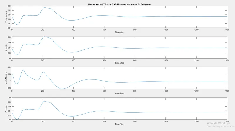
Conservative form
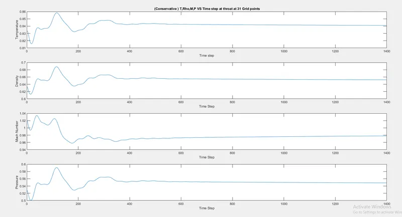
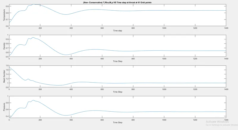
We can observe that the steady results are obtained from around 500 timesteps .
Non-conservative form
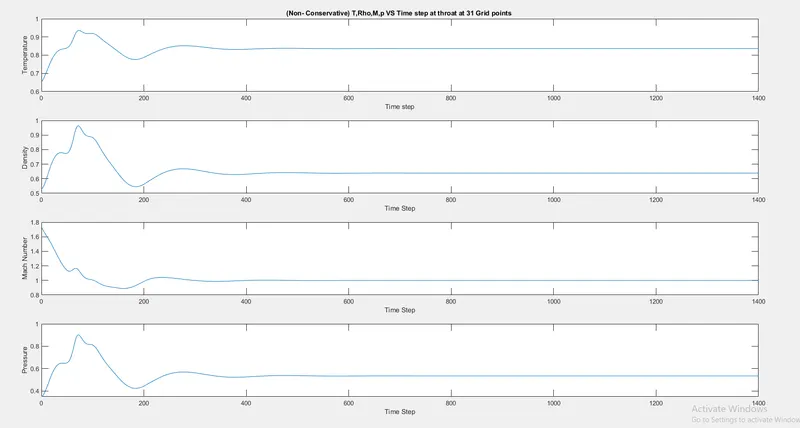
We can observe that the steady results are obtained from around 500 timesteps .
2)Steady-state distribution of primitive variables inside the nozzle
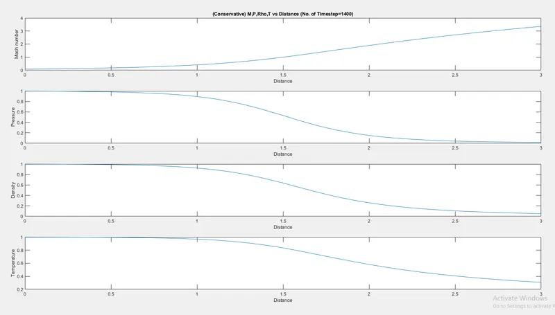
Conservative form
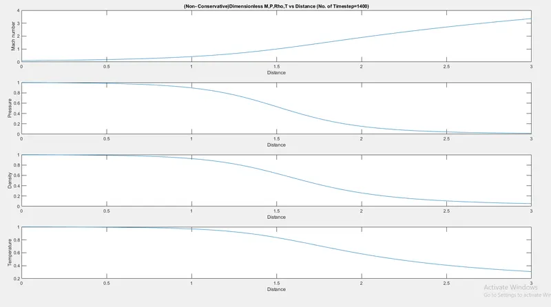
Non Conservative form
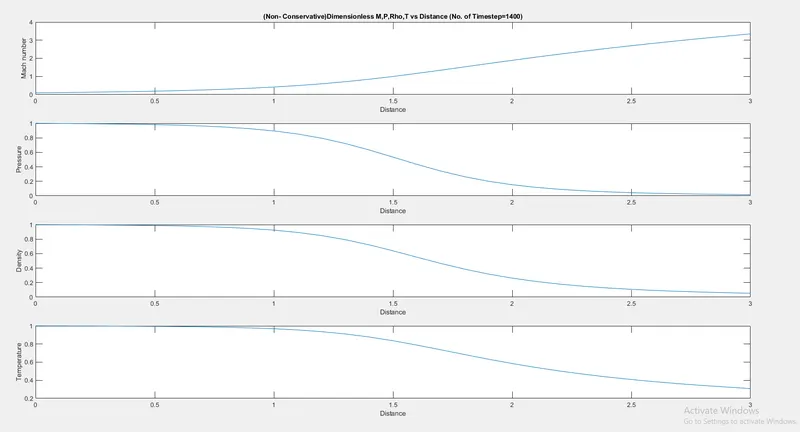
We can observe from the above two graphs that , Velocity increases from inlet to outlet at the expense of pressure drop. Density and temperature drop from inlet to outlet as well .
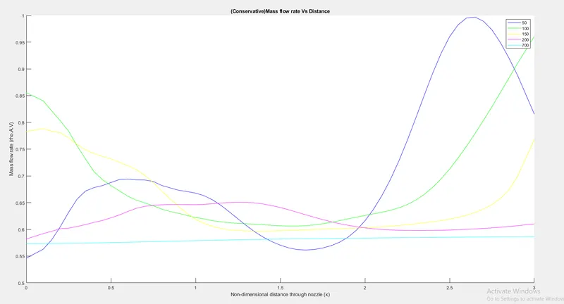
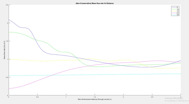
3) Variation of Mass flow rate distribution inside the nozzle at different time steps during the time-marching process
Conservative form
Non-conservative form
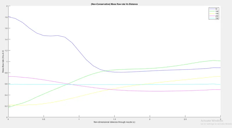
From above two graphs, we can see that conservative form seems to produce more consistent results when it comes to mass flow . In case of non-conservative graph, we note that results show huge variation near initial and final values .
4)Comparison of Normalized mass flow rate distributions of both forms
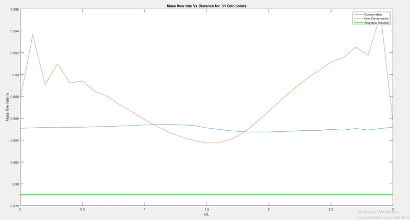
Plots for n=61 .
Inference :
1) Grid independence test
Mass flow rate for 61 grid points .
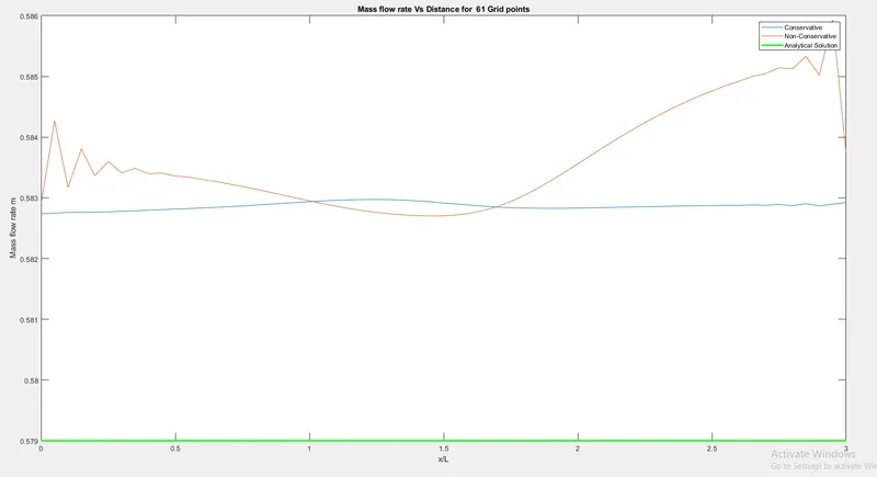
Table for comparison of variables in both cases i.e n=31 and n=61
| Sl No | n=31 | n=61 |
| Conservative | @throat :n=16 | @throat: n=31 |
|
Pressure |
0.5487 | 0.5340 |
| Velocity | 0.8969 | 0.9121 |
| Temperature | 0.8410 | 0.8355 |
| Density | 0.6524 | 0.6391 |
| Mach number | 0.9780 | 0.9979 |
| Non-Conservative | ||
| Pressure | 0.5342 | 0.5327 |
| Velocity | 0.9140 | 0.9138 |
| Temperature | 0.8365 | 0.8345 |
| Density | 0.6378 | 0.6377 |
| Mach Number | 0.9994 | 0.9998 |
We can observe that , as we increase the number of grid points , the steady state numerical results get slightly closer to analytical value .
2) From Conservative and Non-conservative perspective, we can oberve the following
a) Conservation form yields a better mass flow distribution or conservation of mass . We can observe this from the mass flow rate Vs Time step graph or Mass flow rate vs distance graph , where the results seems to be more consistent for conservative form . The conservative form tends to maintain a consisitent line , and has less deviation that non-conservative form .
b) Non-conservative form leads to a smaller residual . Non-conservative form does a better job in the sense that residual decay is an index of quality of numerical algorithm .
c) Non-conservative form seems to produce slightly more accurate results for primitive variables and conservative form seems to produce more accurate results for flux variables . The results in either case are satisfactory .
d) Conservative form requires more calculation time due to decoding of primitive variables to flux variables .