Week 7 - Simulation of a 1D Super-sonic nozzle flow simulation using Macormack Method
THEORY:
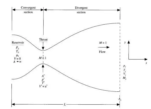
The nozzle has three different parts
Convergent
Divergent
Nozzle
In the convergent part, the Mach number is less than 1 so the fluid particles travel at a speed less than the speed of sound.
In the divergent section, the Mach number is greater than 1 so fluid particles travel at a speed greater than the speed of sound.
Between convergent and divergent section nozzle is there and Mach number is equal to one to fluid particles travels at the speed of sound.
MACH Number: It is defined as the ratio of the speed of flow velocity past boundary to the local speed of sound.
It is a dimensionless number.
`M = v/(root_t)`
where v is the velocity of flow
t is the speed of sound.
Understanding MacCormack method
The MacCormack Method is a variation of the Lax-Wendroff scheme but is much simpler in the application.
The application is done in two steps
1. Predictor step
2. Corrector step
- Predictor step: It uses a forward scheme to determine the value of the certain variable at time step `n+1`.
- Corrector step: This step corrects the values of the variable found in the predictor step but uses a backward scheme.
For non-conservative from:
Predictor method:
Continuity equation:
`((delrho)/(delt))_p = -rho((v_(j+1)-v_j)/dx) - rhov(log(a_(j+1))-log(a_j))/dx - v(rho_(j+1)-rho_j)/dx`
Momentum equation:
`((dv)/(dt))_p = -v.((v_(i+1)-v_(i))/dx) - 1/gamma.((t_(i+1)-t_(i))/dx + t/rho.(rho_(i+1)-rho_(i))/dx)`
energy equation:
`((dT)/(dt))_p = -v.((t_(i+1)-t_i)/dx)- (gamma-1).t.((v_(i+1)-v_i)/dx + v.(loga_(a+1)-loga_(i))/dx)`
Corrector Method:
Continuity equation:
`((delrho)/(delt))_c = -rho((v_(j)-v_(j-1))/dx) - rhov(log(a_(j))-log(a_(j-1)))/dx - v(rho_(j)-rho_(j-1))/dx`
Momentum equation:
`((dv)/(dt))_c = -v.((v_(i)-v_(i-1))/dx) - 1/gamma.((t_(i)-t_(i-1))/dx + t/rho.(rho_(i)-rho_(i-1))/dx)`
Energy equaiton
`((dT)/(dt))_c= -v.((t_(i)-t_(i-1))/dx)- (gamma-1).t.((v_(i)-v_(i-1))/dx + v.(loga_(a)-loga_(i-1))/dx)`
Now The average time derivative:
`((delrho)/(delt)) = 0.5(((delrho)/(delt))_p+ ((delrho)/(delt))_c)`
`((delv)/(delt)) = 0.5(((delv)/(delt))_p+ ((delv)/(delt))_c)`
`((delT)/(delt)) = 0.5(((delT)/(delt))_p+ ((delT)/(delt))_c)`
For conservation form:
Predictor step
Continuity Equation:
`((dU1)/dt)_p = -((F1_(i+1) - F1(i)))/dx`
Momentum Equation:
`((dU2)/dt)_p = -((F2_(i+1) - F2(i)))/dx + J2`
Where
Source term J2 is:
`J2 = 1/gamma.rho.T.(a_(i+1)-a_i)/dx`
Energy equation:
`((dU3)/dt)_p = -((F3_(i+1) - F3(i)))/dx`
Corrector Method:
Continuity Equation:
`((dU1)/dt)_c = -((F1_(i) - F1(i-1)))/dx`
Momentum Equation:
`((dU2)/dt)_c = -((F2_(i) - F2(i-1)))/dx + J2`
Where
Source term J2 is:
`J2 = 1/gamma.rho.T.(a_(i)-a_(i-1))/dx`
Energy equation:
`((dU3)/dt)_c = -((F3_(i) - F3(i-1)))/dx`
NOTE:
In conservation you cant write governing equation in terms of the dependent variable (whose numerical value can be directly be found ) because even if you do so the solution will become unstable spontaneously.
Flux Vectors-
F1 = U2
`F2 = (U2^2)/(U1) + (gamma-1)/gamma.(U3-gamma/2 .(U2^2)/(U1) )`
`F3 = gamma.U2.(U3)/(U1) - gamma.(gamma-1)/2.((U2^3)/(U1^2))`
Solution Vectors
`U1 = rhoa`
`U2 = rhoav`
`U3 = rhoa(T/(gamma-1)+gamma/2.v^2)`
where
`rho`is density
a is the area
v is the velocity
T is temperature
`gamma`is the ratio of specific heat
Average Time derivative
`((delU1)/(delt)) = 0.5(((delU1)/(delt))_p+ ((delU1)/(delt))_c)`
`((delU2)/(delt))_(avg) = 0.5(((delU2)/(delt))_p+ ((delU2)/(delt))_c)`
`((delU3)/(delt))_(avg) = 0.5(((delU3)/(delt))_p+ ((delU3)/(delt))_c)`
For non-conservative form:
Initital conditions:
Values of rho,v,T depends on the position of 'x'
rho = 1-0.3146x
v = 1-0.2341x
T = 1.09x`T ^0.5`
Nozzle shape:
Profile for area 'a':
a = 1+2.2(x-1.5)^2 0<x<3
Mach Number:
`M = v/(root_t)`
For calculation of time step for both of the forms:
`Deltat = c(Deltax)/(a+v)`
where c is courant number
Boundary condition
Subsonic inflow boundary
v1 = 2v2-v3
density and temperature are fixed, rho=1,T=1.
Supersonic Outflow boundary
v(n) = 2.v(n-1) - v(n-2)
rho(n) = 2.rho(n-1) - rho(n-2)
T(n) = 2.T(n-1) - T(n-2)
For Conservative form:
Shape of nozzle and hence area remains same:
a = 1+2.2(x-1.5)^2 0<x<3
Initaial condition:
for 0<x<0.5 rho = 1 and t = 1;
for 0.5<x<1.5 rho =1.0-0.366(x'-0.5) and T'=1.0-0.167(x'-0.5)
for 1.5<x'<3.0: rho'=0.634-0.3879(x'-1.5) and T'=0.8330-3507(x'-1.5)
for the initial condition only,lets assume a constant mass flow through the nozzle and calculate V as,
`v = 0.59/(rhoa)`
Boundary condition
Subsonic inflow boundary
Two properties are held fixed and one is allowed to float rho and T are fixed and V is allowed to float.
`U1_1 = rho a_1`
`U2_2 = 2U2_2 - U2_3`
`U3_1 = rho(e/(gamma-1) + gamma/2v^2)a`
Supersonic outflow boundary
All properties are allowed to float
`U1 = 2U1_(n-1) - U1_(n-2)`
`U2 = 2U2_(n-1) - U2_(n-2)`
`U3 = 2U3_(n-1) - U3_(n-2)`
Diagram of nozzle:
main program:
clear all
close all
clc

%Grid Points
n = 31;
x = linspace(0,3,n);

%Grid Spacing
dx = x(2)-x(1);

%Area
a = 1 + 2.2*(x-1.5).^2;

gamma =1.4;
nt = 1400;
C = 0.5;

%Calling function for non conservative form
tic
[rho_c,t_c,v_c,P_c,M_c,rho_throat_c,v_throat_c,t_throat_c,P_throat_c,M_throat_c,massflow_c,residual_c] = conservation
Time_non_con = toc;

tic
[rho,t,v,P,M,massflow_nc,rho_throat,M_throat,P_throat,t_throat,v_throat,residual] = non_conservation
 Time_con = toc;

%Plots
%Conservation Form
figure(1)
subplot(4,1,1)
plot(x,M_c)
ylabel('Mach Number')
title('Conservation from ')
subplot(4,1,2)
plot(x,P_c)
ylabel('Pressure ratio')
subplot(4,1,3)
plot(x,rho_c)
ylabel('Density ratio')
subplot(4,1,4)
plot(x,t_c)
ylabel('Temperature ratio')
xlabel('x/L')

figure(2)
subplot(4,1,1)
plot(x,M)
ylabel('Mach Number')
title('Non-Conservation from ')
subplot(4,1,2)
plot(x,P)
ylabel('Pressure ratio')
subplot(4,1,3)
plot(x,rho)
ylabel('Density ratio')
subplot(4,1,4)
plot(x,t)
ylabel('Temperature ratio')
xlabel('x/L')

%Plots of flow parameter at throat section
figure(3)
subplot(4,1,1)
plot(1:nt,M_throat_c)
hold on
plot(1:nt,M_throat)
grid on
ylabel('Mach number')
legend('Non-Conservtive','Conservtive')
title('Throat section of nozzle')
subplot(4,1,2)
plot(1:nt,P_throat_c)
hold on
plot(1:nt,P_throat)
grid on
ylabel('P/Po')
legend('Non-Conservtive','Conservtive')
subplot(4,1,3)
plot(1:nt,t_throat_c)
hold on
plot(1:nt,t_throat)
grid on
ylabel('t/t0')
legend('Non-Conservtive','Conservtive')
subplot(4,1,4)
plot(1:nt,rho_throat_c)
hold on
plot(1:nt,rho_throat)
grid on
ylabel('P/Po')
legend('Non-Conservtive','Conservtive')

%Plots of residual
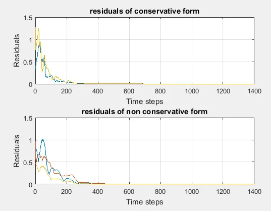
figure(4)
subplot(2,1,1)
plot(1:nt,residual_c)
grid on
xlabel('Time steps')
ylabel('Residuals')
title('residuals of conservative form')
subplot(2,1,2)
plot(1:nt,residual)
grid on
xlabel('Time steps')
ylabel('Residuals')
title('residuals of non conservative form')

%Plot for variation of non dimensional mass flow rate-steady
%state:non-conservative vs conservative
figure(5)
plot(x,massflow_nc(50,:))
hold on
grid on
grid minor
plot(x,massflow_nc(100,:))
plot(x,massflow_nc(150,:))
plot(x,massflow_nc(200,:))
plot(x,massflow_nc(500,:))
plot(x,massflow_nc(700,:))
plot(x,massflow_nc(1400,:))
xlabel('x/L')
ylabel('rhoAV/rho_oA_o_v_o')
legend('50 delta','100 delta','150 delta','200 delta','500 delta','700 delta','1400delta')
title('variation of non dimensional mass flow rate:non-conservative form')

figure(6)
plot(x,massflow_c(50,:))
hold on
grid on
grid minor
plot(x,massflow_c(100,:))
plot(x,massflow_c(150,:))
plot(x,massflow_c(200,:))
plot(x,massflow_c(500,:))
plot(x,massflow_c(700,:))
plot(x,massflow_c(1400,:))
xlabel('x/L')
ylabel('rhoAV/rho_oA_o_v_o')
legend('50 delta','100 delta','150 delta','200 delta','500 delta','700 delta','1400delta')
title('variation of non dimensional mass flow rate: Conservative form')

figure(7)
plot(x,0.587*ones(length(x),1))
hold on
grid on
grid minor
plot(x,massflow_c(end,:))
hold on
plot(x,massflow_nc(end,:))
xlabel('x/L')
ylabel('rhoAv/rho_oA_ov_o')
legend('Exact','Non-conservative','Conservative')
title('Variation of non-dimensional mass flow rate:steady state')
Function of conservation form of governing equation:
function[rho_c,t_c,v_c,P_c,M_c,rho_throat_c,v_throat_c,t_throat_c,P_throat_c,M_throat_c,massflow_c,residual_c] = conservation

n =31;
x = linspace(0,3,n);
dx = x(2)-x(1);

gamma = 1.4;
C = 0.5;

%area
a = 1 + 2.2*(x-1.5).^2;

% %  %Initial conditions
% %  rho = zeros(1,length(x));
% %  t = rho;
% %
% % v = rho;
dt = 0.0267;

nt = 1400;
for i=1:length(x)
    if x(i) >= 0 && x(i) <=0.5
        rho_c(i) = 1;
        t_c(i) = 1;
    elseif x(i) >= 0.5 && x(i) <=1.5
        rho_c(i) = 1-0.366*(x(i)-0.5);
        t_c(i) = 1-0.167*(x(i)-0.5);

    elseif x(i) >= 1.5 && x(i) <=3.5
        rho_c(i) = 0.634-0.3879*(x(i)-1.5);
        t_c(i) = 0.833-0.3507*(x(i)-1.5);
    end
end

v_c = 0.59./(rho_c.*a);
%Mass flow rate
massflow_c = zeros(nt,length(x));

%Defining area of throat
throat = find(a==1)


 %Initial condition for solution vector 'U'
U1 = rho_c.*a;
U2 = rho_c.*a.*v_c;
U3 = rho_c.*a.*(t_c./(gamma-1) + (gamma./2).*(v_c.^2));


for k=1:nt

    U1_old = U1;
    U2_old = U2;
    U3_old = U3;

    %CFL condition
    % dt=min(C*dx./(t.^0.5+v));

    %Initial condition for flux vector 'F'

    F1 = U2;
    F2 = (U2.^2)./U1 + ((gamma-1)/gamma)*(U3 - 0.5*gamma*(U2.^2)./U1);
    F3 = gamma.*(U2.*U3)./(U1) - (gamma*(gamma-1)/2)*(U2.^3)./(U1.^2);

    %Predictor step
    for i=2:length(x)-1

        %Source vector'J'
        J2= (1/gamma)*rho_c(i)*t_c(i)*((a(i+1)-a(i))/dx);

        dU1dt_p(i) = -(F1(i+1)-F1(i))/dx;
        dU2dt_p(i) = -(F2(i+1)-F2(i))/dx + J2;
        dU3dt_p(i) = -(F3(i+1)-F3(i))/dx;

        %Solution update
        U1(i) = U1(i) + dU1dt_p(i)*dt;
        U2(i) = U2(i) + dU2dt_p(i)*dt;
        U3(i) = U3(i) + dU3dt_p(i)*dt;

    end

    F1 = U2;
    F2 = (U2.^2)./U1 + ((gamma-1)/gamma)*(U3 - 0.5*gamma*(U2.^2)./U1);
    F3 = gamma*(U2.*U3)./(U1) - (gamma*(gamma-1)/2)*(U2.^3)./(U1.^2);

        %Obtaining our primitive variable from our solution vectors "U"
        rho_c = U1./a;
        v_c = U2./U1;
        t_c = (gamma-1)*((U3./U1)- ((gamma/2)*(v_c.^2)));

        %Corrector step
        for i=2:length(x)-1
            %Discritizing using backward scheme
            %Source vector'J'
            J2= (1/gamma)*rho_c(i)*t_c(i)*((a(i)-a(i-1))/dx);

            dU1dt_c(i) = -(F1(i)-F1(i-1))/dx;
            dU2dt_c(i) = -(F2(i)-F2(i-1))/dx + J2;
            dU3dt_c(i) = -(F3(i)-F3(i-1))/dx;

        end

        %Computing the average
        dU1dt = 0.5*(dU1dt_p + dU1dt_c);
        dU2dt = 0.5*(dU2dt_p + dU2dt_c);
        dU3dt = 0.5*(dU3dt_p + dU3dt_c);

        residual_c(k,1) = max(abs(dU1dt));
        residual_c(k,2) = max(abs(dU2dt));
        residual_c(k,3) = max(abs(dU2dt));

        %Final solution update
        for j=2:length(x)-1
            U1(j)= U1_old(j) + dU1dt(j)*dt;
            U2(j)= U2_old(j) + dU2dt(j)*dt;
            U3(j)= U3_old(j) + dU3dt(j)*dt;
        end

        %subsonic inflow boundary
        U1(1) = rho_c(1)*a(1);
        U2(1) = 2*U2(2)- U2(3);
        v_c(1) = U2(1)/U1(1);
        U3(1) = U1(1)*((t_c(1)/(gamma-1)) + 0.5*gamma*v_c(1)^2);

        %Supersonic outslow boundary
        U1(end) = 2*U1(end-1) - U1(end-2);
        U2(end) = 2*U2(end-1) - U2(end-2);
        U3(end) = 2*U3(end-1) - U3(end-2);

        %Final values of various variable
        rho_c  = U1./a;
        v_c = U2./U1;
        t_c = (gamma-1)*((U3./U1) - 0.5*gamma*v_c.^2);
        P_c = rho_c.*t_c;
        M_c = v_c./t_c.^0.5;

        massflow_c(k,:) = rho_c.*a.*v_c;

        rho_throat_c(k) = rho_c(throat);
        v_throat_c(k) = v_c(throat);
        t_throat_c(k) = t_c(throat);
        P_throat_c(k) = P_c(throat);
        M_throat_c(k) = M_c(throat);


end


end
Function for a non-conservation form of governing equation:
function[rho_c,t_c,v_c,P_c,M_c,rho_throat_c,v_throat_c,t_throat_c,P_throat_c,M_throat_c,massflow_c,residual_c] = conservation

n =31;
x = linspace(0,3,n);
dx = x(2)-x(1);

gamma = 1.4;
C = 0.5;

%area
a = 1 + 2.2*(x-1.5).^2;

% %  %Initial conditions
% %  rho = zeros(1,length(x));
% %  t = rho;
% %
% % v = rho;
dt = 0.0267;

nt = 1400;
for i=1:length(x)
    if x(i) >= 0 && x(i) <=0.5
        rho_c(i) = 1;
        t_c(i) = 1;
    elseif x(i) >= 0.5 && x(i) <=1.5
        rho_c(i) = 1-0.366*(x(i)-0.5);
        t_c(i) = 1-0.167*(x(i)-0.5);

    elseif x(i) >= 1.5 && x(i) <=3.5
        rho_c(i) = 0.634-0.3879*(x(i)-1.5);
        t_c(i) = 0.833-0.3507*(x(i)-1.5);
    end
end

v_c = 0.59./(rho_c.*a);
%Mass flow rate
massflow_c = zeros(nt,length(x));

%Defining area of throat
throat = find(a==1)


 %Initial condition for solution vector 'U'
U1 = rho_c.*a;
U2 = rho_c.*a.*v_c;
U3 = rho_c.*a.*(t_c./(gamma-1) + (gamma./2).*(v_c.^2));


for k=1:nt

    U1_old = U1;
    U2_old = U2;
    U3_old = U3;

    %CFL condition
    % dt=min(C*dx./(t.^0.5+v));

    %Initial condition for flux vector 'F'

    F1 = U2;
    F2 = (U2.^2)./U1 + ((gamma-1)/gamma)*(U3 - 0.5*gamma*(U2.^2)./U1);
    F3 = gamma.*(U2.*U3)./(U1) - (gamma*(gamma-1)/2)*(U2.^3)./(U1.^2);

    %Predictor step
    for i=2:length(x)-1

        %Source vector'J'
        J2= (1/gamma)*rho_c(i)*t_c(i)*((a(i+1)-a(i))/dx);

        dU1dt_p(i) = -(F1(i+1)-F1(i))/dx;
        dU2dt_p(i) = -(F2(i+1)-F2(i))/dx + J2;
        dU3dt_p(i) = -(F3(i+1)-F3(i))/dx;

        %Solution update
        U1(i) = U1(i) + dU1dt_p(i)*dt;
        U2(i) = U2(i) + dU2dt_p(i)*dt;
        U3(i) = U3(i) + dU3dt_p(i)*dt;

    end

    F1 = U2;
    F2 = (U2.^2)./U1 + ((gamma-1)/gamma)*(U3 - 0.5*gamma*(U2.^2)./U1);
    F3 = gamma*(U2.*U3)./(U1) - (gamma*(gamma-1)/2)*(U2.^3)./(U1.^2);

        %Obtaining our primitive variable from our solution vectors "U"
        rho_c = U1./a;
        v_c = U2./U1;
        t_c = (gamma-1)*((U3./U1)- ((gamma/2)*(v_c.^2)));

        %Corrector step
        for i=2:length(x)-1
            %Discritizing using backward scheme
            %Source vector'J'
            J2= (1/gamma)*rho_c(i)*t_c(i)*((a(i)-a(i-1))/dx);

            dU1dt_c(i) = -(F1(i)-F1(i-1))/dx;
            dU2dt_c(i) = -(F2(i)-F2(i-1))/dx + J2;
            dU3dt_c(i) = -(F3(i)-F3(i-1))/dx;

        end

        %Computing the average
        dU1dt = 0.5*(dU1dt_p + dU1dt_c);
        dU2dt = 0.5*(dU2dt_p + dU2dt_c);
        dU3dt = 0.5*(dU3dt_p + dU3dt_c);

        residual_c(k,1) = max(abs(dU1dt));
        residual_c(k,2) = max(abs(dU2dt));
        residual_c(k,3) = max(abs(dU2dt));

        %Final solution update
        for j=2:length(x)-1
            U1(j)= U1_old(j) + dU1dt(j)*dt;
            U2(j)= U2_old(j) + dU2dt(j)*dt;
            U3(j)= U3_old(j) + dU3dt(j)*dt;
        end

        %subsonic inflow boundary
        U1(1) = rho_c(1)*a(1);
        U2(1) = 2*U2(2)- U2(3);
        v_c(1) = U2(1)/U1(1);
        U3(1) = U1(1)*((t_c(1)/(gamma-1)) + 0.5*gamma*v_c(1)^2);

        %Supersonic outslow boundary
        U1(end) = 2*U1(end-1) - U1(end-2);
        U2(end) = 2*U2(end-1) - U2(end-2);
        U3(end) = 2*U3(end-1) - U3(end-2);

        %Final values of various variable
        rho_c  = U1./a;
        v_c = U2./U1;
        t_c = (gamma-1)*((U3./U1) - 0.5*gamma*v_c.^2);
        P_c = rho_c.*t_c;
        M_c = v_c./t_c.^0.5;

        massflow_c(k,:) = rho_c.*a.*v_c;

        rho_throat_c(k) = rho_c(throat);
        v_throat_c(k) = v_c(throat);
        t_throat_c(k) = t_c(throat);
        P_throat_c(k) = P_c(throat);
        M_throat_c(k) = M_c(throat);


end


end
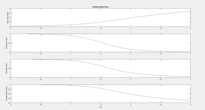
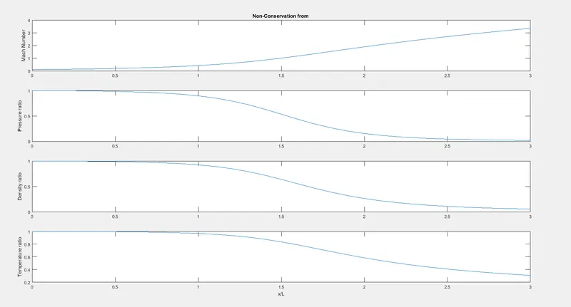
| Non-Con | Con | Non-Con | Con | Non-Con | Con | Non-Con | Con | Non-Con | Con |
| 0 | 0 | 0.098782 | 0.098348 | 1 | 1 | 1 | 1 | 1 | 1 |
| 0.5 | 0.5 | 0.18703 | 0.18564 | 0.98232 | 0.98288 | 0.98734 | 0.98769 | 0.99513 | 0.99513 |
| 1 | 1 | 0.41552 | 0.41592 | 0.89547 | 0.89377 | 0.92414 | 0.92288 | 0.96846 | 0.96846 |
| 1.5 | 1.5 | 0.99937 | 0.98173 | 0.53424 | 0.54635 | 0.63869 | 0.65039 | 0.84005 | 0.84005 |
| 2 | 2 | 1.8901 | 1.9081 | 0.15316 | 0.15316 | 0.26184 | 0.25967 | 0.57992 | 0.57992 |
| 2.5 | 2.5 | 2.6963 | 2.7149 | 0.043785 | 0.043785 | 0.10721 | 0.10582 | 0.40503 | 0.40503 |
| 3 | 3 | 3.3532 | 3.367 | 0.016295 | 0.016295 | 0.052857 | 0.052717 | 0.30549 | 0.30549 |
From the above plot and data, we can notice that as the match number increases flow reaches from subsonic to the supersonic regime the primitive variable: pressure, density, and temperature shows declivity after the sonic region till the exit of the nozzle. Although these results are almost identical to the analytical solution results validated from the CFD book by Jhon D Anderson.
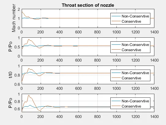
From the above results, we can say that the conservative form converges to the steady-state faster than the non-conservative form.
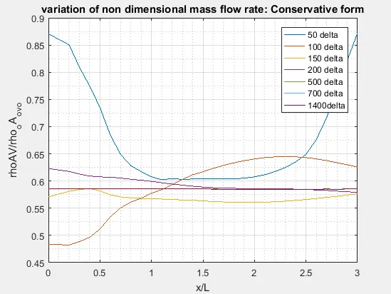
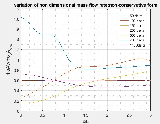
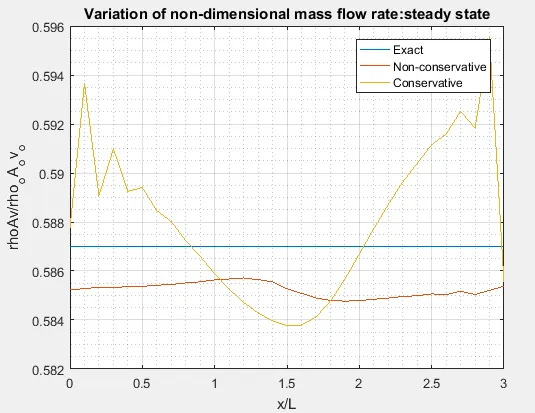
In the above plot, we compare the steady-state variations of mass flow obtained with the non-conservative and conservative forms of the governing equations. Here we see that the steady-state mass flow distribution predicted by the conservative form of the equation is much more satisfactory than that obtained from the non-conservative form on the two accounts.
1. The conservative from gives a distribution ie., much closer to being a constant. In contrast, the non-conservative results have a sizeable variation with some oscillations at both the inflow and outflow boundary if the course on a practical basis these variations are not apparent and the mass flow essentially appears to be constant.
2.The steady state mass flow results obtained with the conservative form are on the whole much closer to the exact analytical solution.
| Grid dependency test | rho/rhoO | T/To | P/Po | M |
| exact analytical solution | 0.634 | 0.833 | 0.528 | 1 |
| non-conservative form 31 grids | 0.6387 | 0.8365 | 0.5342 | 0.9994 |
| conservative form 31 grids | 0.6504 | 0.8401 | 0.5465 | 0.9817 |
| non-conservative form 61 grids | 0.6376 | 0.8354 | 0.5326 | 0.9997 |
| conservative form 61 grids | 0.6382 | 0.8352 | 0.5330 | 0.9993 |
The time taken for non-conservative form 31 grids points is 0.0755 sec and for 61 grid points 0.1041sec
Time taken for conservative form 31 grid points is 0.1130 sec and for 61 grid points is 0.1478sec