Week 5 - Mid term project - Solving the steady and unsteady 2D heat conduction problem
Solving using steady-state:
In a steady-state, the temperature within the body doesn't change with time.
The equation for steady-state conduction is as follow:
`(del(T))/(del(x^2)) + (del(T))/(del(y^2)) = 0`
Discritizing the above equation with equal grid points and `dx = dy` we get

Steady State :
Main Program
clear all
close all
clc

%Defiining all the parameters(constans)
nx = 10;
ny = nx;

L =1;
x = linspace(0,1,nx);
y = linspace(0,1,ny);

dx = x(2) - x(1);
dy = y(2) - y(1);

%Absolute error
error = 9e9;
tol = 1e-4;

%SOR method
omega = 2/(1+sin(pi*dx));

%Defining Boundary Condition
temp = ones(nx,ny);

temp_top = 600;
temp_bottom = 900;
temp_left = 400;
temp_right = 800;

temp(:,1) = temp_left;
temp(:,end) = temp_right;
temp(end,:)= temp_bottom;
temp(1,:) = temp_top;
temp_old = temp;


iterative_solver = input('1. Jacobi, 2. Gauss Seidel, 3.SOR  \nEnter a value for the type of solver: \n')

if iterative_solver == 1;
    %Jacobi Method
    jt = 0;

    while (error>tol)

    for i=2:nx -1
        for j = 2:ny -1
            temp(i,j) = 0.25 * (temp_old(i-1,j)+temp_old(i+1,j)+ temp_old(i,j+1)+temp_old(i,j-1));
        end
    end
    error = max(max(abs(temp_old-temp)));
    temp_old = temp;
    jt = jt+1;


    end
    %Plotting
    figure(1)
    contourf(x,fliplr(y),temp,'ShowText','ON');
    colorbar
    text = sprintf('Jacobi Iteration = %d ',jt)
    title(text);
    xlabel('X axis');
    ylabel('Y axis');
    pause(0.0001);
end

if iterative_solver == 2;

    %Gauss sedial method
    gs = 0;
    while (error>tol)

        for i=2:nx -1
            for j = 2:ny -1
            temp(i,j) = 0.25 * (temp(i-1,j)+temp_old(i+1,j)+ temp_old(i,j+1)+temp(i,j-1));
            end
        end
    gs = gs+1;
    error = max(max(abs(temp_old-temp)));
    temp_old = temp;


    end
    %Plotting
    figure(2)
    contourf(x,fliplr(y),temp,'ShowText','ON');
    colorbar
    text = sprintf('Gauss Sedial = %d',gs)
    title(text);
    xlabel('X axis');
    ylabel('Y axis');
    pause(0.0001);
end

if iterative_solver == 3;
    sor = 0;
    while (error>tol)

        for i=2:nx -1
            for j = 2:ny -1
                temp(i,j) = ((1-omega)*temp_old(i,j))+ (0.25*omega*(temp(i-1,j)+temp_old(i+1,j)+ temp_old(i,j+1)+temp(i,j-1)));
            end
        end
        error = max(max(abs(temp_old-temp)));
        temp_old = temp;
        sor = sor + 1;

    end
        %Plotting
        figure(3)
        contourf(x,fliplr(y),temp,'ShowText','ON');
        colorbar
        pause(0.0001);
        text = sprintf('SOR iteration = %d',sor);
        title(text);
        xlabel('X axis');
        ylabel('Y axis');

end
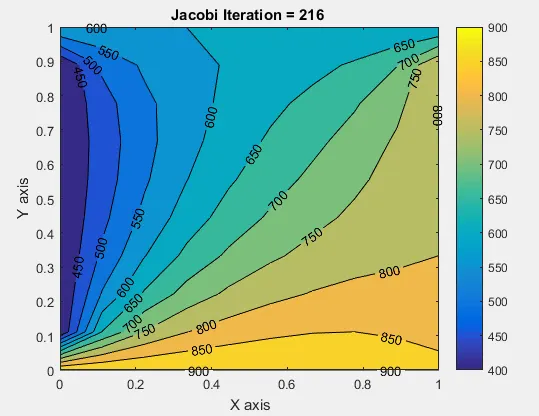
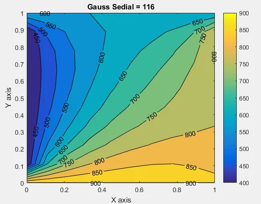
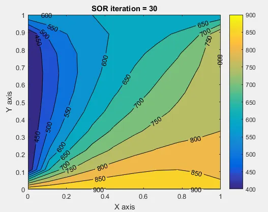
Plots Obtained are:
Jacobi Method:
Gauss Sedial Method:
SOR Method:
Unsteady State: In the unsteady state temperature within the body does change with time
The equation for unsteady state is as follow:
`(delT)/(delt) = alpha(((del^2 T)/(delx^2))+((del^2 T)/(dely^2)))`
Discretizing the above equation we get
`(T^(n+1))_(i,j)=(T^(n))_(i,j)+K1((T^(n+1))_(i-1,j)-2(T^(n+1))_(i,j)+(T^(n+1))_(i+1,j))+K2((T^(n+1))_(i,j-1)-2(T^(n+1))_(i,j)+(T^(n+1))_(i,j+1))`
`(T^(n+1))_(i,j)=((T^(n))_(i,j)+(K1(T_(i-1,j)+T_(i+1,j))+K2(T_(i,j-1)+T_(i,j+1)))^(n+1))/(1+2K1+2K2)`
where
`k_1 = alpha ((Deltat)/(Deltax^2))`
`k_2 = alpha ((Deltat)/(Deltay^2))`
where
'n' denotes time index
'i' and 'j' denotes space index
Program(Explicit Method)
This method involves solving an equation using current and later state of the system.
    clear all
    close all
    clc

    %Defining all the necessesary parameters
    L = 1;
    nx = 30;
    ny = nx;
    x = linspace(0,L,nx);
    y = linspace(0,L,ny);
    dx = x(2)-x(1);
    dy = dx;
    %Absolute term
    error = 9e9;
    tol = 1e-4;

    dt = 0.1;

    %Thermal Conductivity
    alpha = 1e-3;

    %CFL Number
    k1 = alpha*dt/(dx^2);
    k2 = k1;

    %Creating Temperature Matrix(Initial)
    temp = ones(nx,ny);
    temp_top = 600;
    temp_bottom = 900;
    temp_left = 400;
    temp_right = 800;

    temp(:,1) = temp_left;
    temp(:,end) = temp_right;
    temp(end,:)= temp_bottom;
    temp(1,:) = temp_top;
    temp_old = temp;

    a = 0;

    for nt = 1:1400
        for i = 2:nx-1
            for j = 2:ny-1


                temp(i,j) = temp_old(i,j)+ k1*(temp_old(i-1,j) -2*temp_old(i,j) + temp_old(i+1,j)) +k2*(temp_old(i,j-1) -2*temp_old(i,j) + temp_old(i,j+1));
            end
        end

            error = max(abs(temp_old-temp));
            temp_old =  temp;
            a = a+1;


    end
    contourf(x,flip(y),temp,'ShowText','ON')
    colorbar
    title_text=sprintf('Explicit method ,Iteration number=%d',a);
    title(title_text)
    xlabel('X axis');
    ylabel('Y axis');
Plot obtained
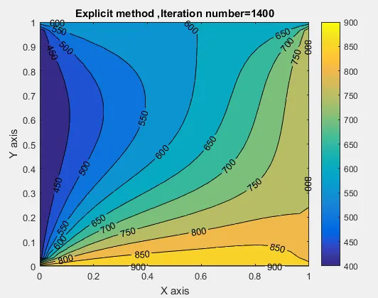
Explicit Method:
This method is used to calculate the state of a given system at a different time from the current time.
Program used is:
clear all
close all
clc

%Number of grid points
nx = 50;
ny = nx;


L =1;
x = linspace(0,1,nx);
y = linspace(0,1,ny);

dx = x(2) - x(1);
dy = y(2) - y(1);

dt = 10;

%Thermal conductivity
alpha = 2;

%Absolute Error
error_1 = 9e9;
tol = 1e-5;

%CFL number
k1 = alpha*dt/(dx^2);
k2 = k1;

rf = 1.8;

%Initial temperature array
%Boundary conditions
temp_top = 600;
temp_bottom = 900;
temp_left = 400;
temp_right = 800;

temp = ones(nx,ny);

temp(:,1) = temp_left;
temp(:,end) = temp_right;
temp(end,:)= temp_bottom;
temp(1,:) = temp_top;
temp_old = temp;
temp_prev = temp;

%SOR (magnification factor)
omega = 2/(1+sin(pi*dx));


%Jacobi Method
s_iter = 0;
t_iter =0;
error_2 = error_1;
iterative_solver = input('1. Jacobi, 2. Gauss Seidel, 3.SOR \nEnter a value for the type of solver: \n');
tic
if iterative_solver == 1
     while(error_2>=tol)
         %Convergence loop
        while(error_1>tol)
            %Space loop
            for i = 2:nx-1
                for j = 2:ny-1
                    term_1 = (1+(2*k1)+(2*k2))^-1;
                    term_2 = k1*term_1;
                    term_3 = k2*term_1;
                    h = temp_old(i-1,j) + temp_old(i+1,j);
                    v = temp_old(i,j-1) + temp_old(i,j+1);
                    temp(i,j) = (term_1*temp_prev(i,j) + term_2*h + term_3*v);
                end
            end
            error_1 = max(max(abs(temp_old - temp)));
            temp_old = temp;
            s_iter = s_iter+1;
        end
        error_2 = max(max(abs(temp_prev - temp)));
        temp_prev = temp;
        t_iter = t_iter+1;
     end
end


if iterative_solver == 2
     while(error_2>=tol)
         %Convergence loop
        while(error_1>tol)
            %Space loop
            for i = 2:nx-1
                for j = 2:ny-1
                    term_1 = (1+(2*k1)+(2*k2))^-1;
                    term_2 = k1*term_1;
                    term_3 = k2*term_1;
                    h = temp(i-1,j) + temp_old(i+1,j);
                    v = temp(i,j-1) + temp_old(i,j+1);
                    temp(i,j) = (term_1*temp_prev(i,j) + term_2*h + term_3*v);
                end
            end
            error_1 = max(max(abs(temp_old - temp)));
            temp_old = temp;
            s_iter = s_iter+1;
        end
        error_2 = max(max(abs(temp_prev - temp)));
        temp_prev = temp;
        t_iter = t_iter+1;
     end
end


if iterative_solver == 3
    while(error_2>tol)
        s_iter = s_iter + 1;
        while(error_1>tol)
            for i = 2:nx - 1
                for j = 2:ny-1
                    term_1 = (1+(2*k1)+(2*k2))^-1;
                    term_2 = k1*term_1;
                    term_3 = k2*term_1;
                    h = temp(i-1,j) + temp_old(i+1,j);
                    v = temp(i,j-1) + temp_old(i,j+1);
                    temp_end(i,j) = (term_1*temp_prev(i,j) + (term_2*h + term_3*v));
                    temp(i,j) = ((1-omega)*temp_old(i,j)) + (temp_end(i,j)*omega);
                end
            end
            error_1 = max(max(abs(temp_old - temp)));
            temp_old = temp;
            s_iter = s_iter+1;
        end
        error_2 = max(max(abs(temp_prev - temp)));
        temp_prev = temp;
    end

end


time_1 = toc;
%Plotting
figure(1)
contourf(x,fliplr(y),temp,'ShowText','ON');
colorbar
pause(0.1);
text = sprintf(' Iteration: %d\nTime taken: %d',s_iter,time_1);
title(text);
xlabel('X axis');
ylabel('Y axis');
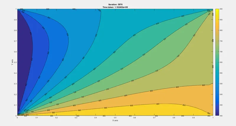
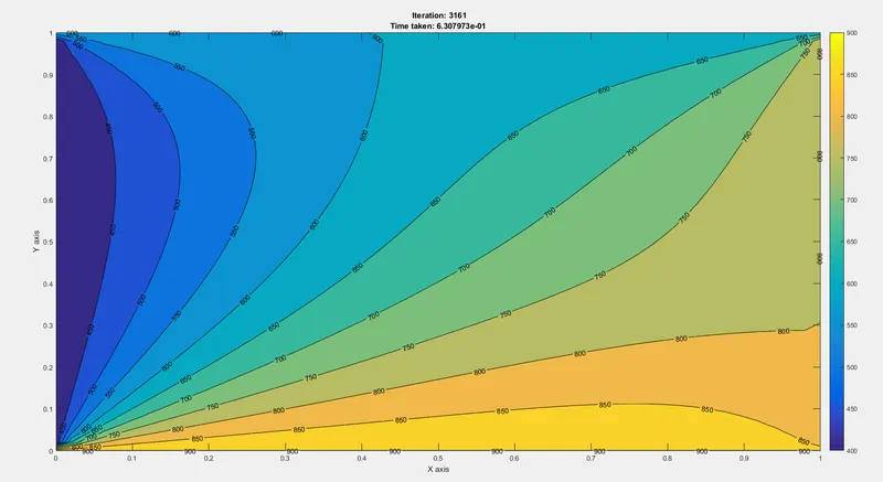
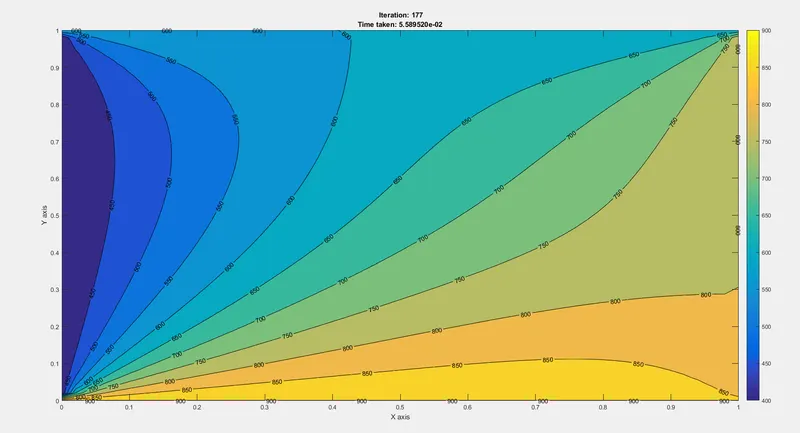
Plots obtained are
jacobi
Gauss Seidel:
SOR method
Results:
From the above plots, we can conclude that SOR methods take the least amount of time and the least number of iterations.
When we talk about the transient state, it takes more computational time to solve their equation.
For CFL number greater that 0.25 we use implicit methods because they are unconditionally stable and for less than 0.25 we can use the explicit method.'
Over all SOR methods are highly effective because of lower number of iterations, time and error value.