Week 3 - Taylor table method and Matlab code

Objective:

Derive the following 4th order approximations of the second-order derivative.

1. Central difference

2. Skewed right-sided difference

3. Skewed left-sided difference

After deriving these schemes, prove that your skewed schemes are fourth-order accurate.

Once you have done this, write a program in Matlab to evaluate the second-order derivative of the analytical function exp(x)*cos(x) and compare it with the 3 numerical approximations that you have derived.

Provide a plot that compares the absolute error between the above-mentioned schemes

In your own words, describe why a skewed scheme is useful? What can a skewed scheme do that a CD scheme cannot?

Derivation:

1. Central Difference:

In order to calculate 4th order approximations of the second-order derivative we first need to find the number of nodes(constants) required on stencils

The order of accuracy P = Number of nodes in the stencil N - order of derivative Q + 1 for symmetric/central schemes

Therefore: N = P+Q - 1

P = 4 ; Q = 2

Therefore N = 5

let these constants be [a, b, c, d, e]

`(d^2f)/(dx^2) = af(a - 2dx) + bf(x - dx) + cf(x) + df(x +dx) + ef(x + 2dx)` let this be equation (1)

These values of the nodes can be coputed by Taylor's Tabel

`(d^2f)/(dx^2)`	`f(x)`	`f'(x)dx`	`(f''(x)dx^2)/(2!)`	`(f'''(x)dx^3)/(3!)`	`(f''''(x)dx^4)/(4!)`	`(f'''''(x)dx^5)/(5!)`	`(f''''''(x)dx^6)/(6!)`
`af(x-2dx)`	a	-2a	4a	-8a	16a	-32a	64a
`bf(x-dx)`	b	-b	b	-b	b	-b	b
`cf(x)`	c	0	0	0	0	0	0
`df(x+dx)`	d	d	d	d	d	d	d
`ef(x+2dx)`	e	2e	4e	8e	16e	32e	64e
`sum row`	0	0	1	0	0	Unknown	Unknown

We have ignored higher-order derivative because for 5 unknown 5 equation are enough.

a + b + c + d + e = 0 ----(2)

-2a -b + 0 + d + 2e = 0 ----(3)

`(dx^2(4a + b + 0 + d + 4e))/(2) = 1` ----(4)

-8a - b + 0 + d + 8e = 0 ----(5)

16a + b +0 + d + 16e = 0 ----(6)

lets omit dx^2 from equation 4 for ease of using matrix computation, it will be included in the next step.

On writing these equations in matrix form, we get:

AX = B

`[[1 ,1, 1, 1, 1 ],[-2, -1, 0 , 1 , 2],[4 , 1 , 0 ,1 , 4],[-8 , -1 , 0 , 1 , 8],[16 , 1, 0 , 1 , 16]]``[[a],[b],[c],[d],[e]]`= `[[0],[0],[2],[0],[0]]`

On solving this matrix we get

`[[a],[b],[c],[d],[e]]` = `[[-0.0833],[1.3333],[-2.5],[1.3333],[-0.0833]]`

From the above answer it is clear that a=e ; b=d , also these values must be devied by `dx^2` as we have previously omitted for ease of calcualtions .

Substituting these values in equation (1)

`(d^2f)/(dx^2) = (-0.0833f(a - 2dx) + 1.3333f(x - dx) + -2.5f(x) + 1.3333f(x +dx) + -0.0833f(x + 2dx))/(dx^2) + ...`

Proof that the above scheme is fourth order scheme:

Lets expand taylor series by, only including higher order terms

`((d^2f)/(dx^2))= (4a + b + 0 + d + 4e)(f''(x)dx^2)/2! + (-32a -b + 0 +d +32e)f'''''(x)dx^2 / 5! + (64a + b + 0 +d +64e)f''''''dx^2/(6!) + ...`

As a=e ; b=d substituting in the above equation we get cofficient of fifth derivative equal to zero and cofficient of f''(x)must be equal to 1

Therefore

`(d^2f)/dx^2 = ((4a +b + 0 +d +4e ) f''(x)dx^2)/(2!) + ((64a+b+0+d+64e)f'''''d(x))/(6!))`

Now substituting the initail value of second derivative

`af(x-2dx)+ bf(x-dx)+cf(x)+df(x+dx)+ef(x+2dx) = ((4a +b + 0 +d +4e ) f''(x)dx^2)/(2!) + ((64a+b+0+d+64e)f'''''dx^6)/(6!))`

Deviding whole equation by `dx^2`

`(af(x-2dx)+ bf(x-dx)+cf(x)+df(x+dx)+ef(x+2dx)) / (dx^2) = ((4a +b + 0 +d +4e ) f''(x)/(2!) + ((64a+b+0+d+64e)f'''''dx^4)/(6!))`

It can be clearly seen that in RHS the dx term has a power of 4, this term is also known as the truncation term or discretization error which indicates the order of approximation.

2.Skewed right side difference:

To compute the fourth-order derivative we first need to find the number of nodes required using the formula

The order of accuracy P = Number of nodes in the stencil N - order of derivative Q for one-sided/skewed schemes

Therefore

N = P + Q ; P = 4 and Q = 2;

N = 6

Let these points be `f(x), f(x + dx), f(x +2dx), f(x +3dx), f(x +4dx), f(x +5dx)`

for "Skewed right side difference" these are defined at the right side of point `x`

Therefore the fourht order approximation of second order derivative of `f` is given by

`(d^2f)/(dx^2) = af(x)+ bf(x + dx)+c f(x +2dx)+ df(x +3dx)+e f(x +4dx)+g f(x +5dx)`

The values of these cofficient can be determined by Taylor's Table

`(d^2f)/(dx^2)`	`f(x)`	`f'(x)dx`	`(f''(x)dx^2)/(2!)`	`(f'''(x)dx^3)/(3!)`	`(f''''(x)dx^4)/(4!)`	`(f'''''(x)dx^5)/(5!)`	`(f''''''(x)dx^6)/(6!)`
`af(x)`	a	0	0	0	0	0	0
`bf(x+dx)`	b	b	b	b	b	b	b
`cf(x+2dx)`	c	2c	4c	8c	16c	32c	64c
`df(x+3dx)`	d	3d	9d	27d	81d	243d	729d
`ef(x+4dx)`	e	4e	16e	64e	256e	1024e	4096e
`gf(x+5dx)`	g	5g	25g	125g	625g	3125g	15625g
`sum rows`	0	0	1	0	0	0	unknown

We get six unknown namely a,b,c,d,e,g therefore we need six equations

`a+b+c+d+e+g = 0`

`0+b+2c+3d+4e+5g= 0`

`dx^2/(2!) *(0 +b+4c+9d+16e+25g)=1`

`0+b+8c+27d+64e+125g = 0`

`0+b+16c+81d+256e+625g= 0`

`0+b+32c+243d+1024e+3125h = 0`

For the same reason as before we are currently ignoring the `dx^2`term

Writing equation in matrix form we get,

AX=B

`[[1,1,1,1,1,1],[0,1,2,3,4,5],[0,1,3,9,16,25],[0,1,8,27,64,125],[0,1,16,81,256,625],[0,1,31,243,1024,3125]]``[[a],[b],[c],[d],[e],[g]]` = `[[0],[0],[2],[0],[0],[0]]`

Solving the above equation we get

`X=``[[a],[b],[c],[d],[e],[g]] = [[3.75],[-12.83333],[17.8333],[-13],[5.0833],[-0.8333]]`

Proof that it is second order error

On expanding Taylor's Table

`(d^2f)/(dx^2) =((0 +b+4c+9d+16e+25g)f''dx^2)/(2!) + ((0+b+64c+729d+4096e+15625g)f''''''dx^6)/(6!))+ ...`

Substituting the value of constants and equating to its initial value we get

`af(x)+bf(x+dx)+cf(x+2dx)+df(x+3dx)+ef(x+4dx)+gf(x+5dx) = f''(x)+ ((0+b+64c+729d+4096e+15625g)f''''''dx^6)/(6!))`

Deviding whole equation by `dx^2` and ignoring higher order terms we get

`(af(x)+bf(x+dx)+cf(x+2dx)+df(x+3dx)+ef(x+4dx)+gf(x+5dx))/(dx^2)= f''(x)+ O(dx^4)`

This proves that the scheme is fourth order accurate.

3.Skewed left side difference:

As mentioned above we first need to find the number of nodes in order to solve skewed left side difference which can be calculated using the formula

The order of accuracy P = Number of nodes in the stencil N - order of derivative Q for one-sided/skewed schemes

N=P+Q; P=4, Q=2;`-125a-64b-27c-8d-e+0=0`

N=6

So there are six nodes which means there are five points around x, let they be dx apart from each other, let these points be `(x-dx),(x-2dx),(x-3dx),(x-4dx),(x-5dx)`

Then the fourth-order left-skewed difference approximation for the second-order derivative is given by

`(d^2f)/(dx^2)= af(x-5dx) + bf(x-4dx)+cf(x-3dx)+ df(x-2dx)+ef(x-dx)+gf(x)`

The values of these cofficient can be determined by the Taylor's Table:

`(d^2f)/(dx^2)`	`f(x)`	`f'(x)dx`	`(f''(x)dx^2)/(2!)`	`(f'''(x)dx^3)/(3!)`	`(f''''(x)dx^4)/(4!)`	`(f'''''(x)dx^5)/(5!)`	`(f''''''(x)dx^6)/(6!)`
`af(x-5dx)`	a	-5a	25a	-125a	625a	-3125a	15625a
`bf(x-4dx)`	b	-4b	16b	-64b	256b	-1024b	4096b
`cf(x-3dx)`	c	-3c	9c	-27c	81c	-243c	729c
`df(x-2dx)`	d	-2d	4d	-8d	16d	-32d	64d
`ef(x-1dx)`	e	-e	e	-e	e	-e	e
`gf(x)`	g	0	0	0	0	0	0
`sum rows`	0	0	1	0	0	0	unknown

We get 5 equations from the Taylor's table

`a+b+c+d+e+g=0`

`-5a-4b-3c-2d-e-0=0`

`(dx^2(25a+16b+9c+4d+e+0))/2 = 0`

`-125a -64b-27c-8d-e+0=0`

`625a+256b+81c+16d+e+0=0`

`-3125a-1024b-243c-32d-e+0=0`

Omitting the dx^2 term as before and writing the equation in matrix form, we get,

AX = B

`[[1,1,1,1,1,1],[-5,-4,-3,-2,-1,0],[25,16,9,4,1,0],[-125,-64,-27,-8,-1,0],[625,256,81,16,1,0],[-3125,-1024,-243,-32,-1,0]][[a],[b],[c],[d],[e],[g]]=[[0],[0],[2],[0],[0],[0]]`

`X=[[a],[b],[c],[d],[e],[g]]=[[-0.8333],[5.08333],[-13],[17.8333],[-12.8333],[3.75]]`

Therefore, fourth order left skewed difference approximation for the second order derivative is given by

`(d^2f)/(dx^2)= (-0.8333f(x-5dx) + 5.08333f(x-4dx)-13f(x-3dx)+ 17.8333f(x-2dx)-12.8333f(x-dx)+3.75f(x))/(dx^2)`

As left and right skewed difference are same but in opposite order therefore for the same reason left side skewed difference is also 4th order scheme, also the values of cofficient is same but in opposite order which is obvious because the points are takken in opposite direction.

Main program:

%Creating a program that computes analytical error with the rest of the methods
%we have learned so far
%Function given to solve, f(x)= exp(x)*cos(x)

clear all
close all
clc

%Providing a random value to solve the equation
x = 2*pi;
dx = linspace(pi/4, pi/400000,60);

%Analytical solution for the given function (2nd order derivative)
analytical_solution = -2*exp(x)*sin(x);

%Creting a matrix to store the values of error
cd_error = zeros(1,length(dx));
sld_error = zeros(1,length(dx));
srd_error = zeros(1,length(dx));

%Creating a loop to calculate various solution of nodes at different points
for i = 1:length(dx)
    f=exp(x)*cos(x);
    f1 = exp(x+dx(i))*cos(x+dx(i));
    f2 = exp(x+2*dx(i))*cos(x+2*dx(i));
    f3 = exp(x+3*dx(i))*cos(x+3*dx(i));
    f4 = exp(x+4*dx(i))*cos(x+4*dx(i));
    f5 = exp(x+5*dx(i))*cos(x+5*dx(i));
    b1 = exp(x-dx(i))*cos(x-dx(i));
    b2 = exp(x-2*dx(i))*cos(x-2*dx(i));
    b3 = exp(x-3*dx(i))*cos(x-3*dx(i));
    b4 = exp(x-4*dx(i))*cos(x-4*dx(i));
    b5 = exp(x-5*dx(i))*cos(x-5*dx(i));
    
    %Solving the equation using multiple differencing schemes
    cd_solution = central_difference(f2, f1, f, b1, b2, dx(i));
    srd_solution = skewed_right_differnce(f,f1, f2, f3, f4, f5, dx(i));
    sld_solution = skewed_left_difference(b5, b4, b3, b2, b1, f, dx(i));
     
    %Computing error in differnt schemes
    cd_error(i) = abs(analytical_solution - cd_solution);
    srd_error(i) = abs(analytical_solution - srd_solution);
    sld_error(i) = abs(analytical_solution -sld_solution);
end
 

%Plotting different solution
loglog(dx,cd_error, dx,srd_error, dx,sld_error);
title('Comparision of Different schemes')
xlabel('dx')
ylabel('Error at x = pi/4');
legend('Central differnce','Skewed Right Differnce','Skewed Left Differnce');

Functions:

%Creating function for Central Differnce
function cd_solution = central_difference(f2, f1, f, b1, b2, dx)

%values of cofficient after solving Taylor's Table
a = -0.0833;
b = 1.3333;
c = -2.5;
d = 1.3333;
e = -0.0833;

cd_solution = (a*f2 + b*f1 + c*f + d*b1 + e*b2)/(dx^2);
end

%Function for Skewed Right Diffence Solution
function srd_solution = skewed_right_differnce(f,f1,f2,f3,f4,f5,dx)
 
%Values of cofficient 
a = 3.7500;
b = -12.83333;
c = 17.83333;
d = -13.0000;
e = 5.08333;
g = -0.83333;

srd_solution = (a*f + b*f1 + c*f2 + d*f3 + e*f4 + g*f5)/(dx^2);
end

%Function for skewed left side differnce
function sld_solution = skewed_left_difference(b5,b4,b3,b2,b1,f,dx)

%Values of the cofficient after solving Taylor's Table
a = -0.83333;
b = 5.08333;
c = -13.0000;
d = 17.83333
e = -12.83333;
g = 3.7500;

sld_solution = (a*b5 + b*b4 +c*b3 + d*b2 + e*b1 + g*f)/(dx^2)
end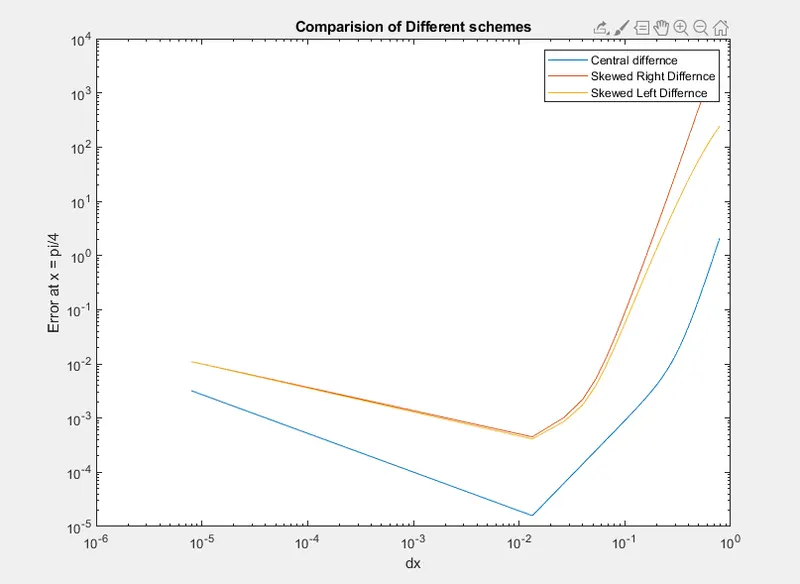

It is clear form the plot that the central differencing scheme is better then both of the skewed left and right differencing schemes, error in both the skewed schemes is higher then the central differencing scheme

Significance of skewed schemes:

Central differencing schemes requires a function to act on both sides of a boundary, so if you want to compute a numerical approximation of a function, central differencing schemes won't always be desired because they will not be executed in the first place, in such a scenario skewed differencing comes to handy where you just need data(nodes) on either side of the boundary hence it enables us to solve numerical approximation which was not possible by solving them in central differencing schemes.