Week 7 - Simulation of a 1D Super-sonic nozzle flow simulation using Macormack Method

Aim: - To write a program in MATLAB to simulate 1-D super sonic nozzle flow using Mac-Cormack’s Method.

Objective: -

1. To plot Steady state distribution of primitive variable inside nozzle for both conservative and Non conservative forms.
2. To plot Time wise variation of primitive variable in Throat region of the Nozzle.
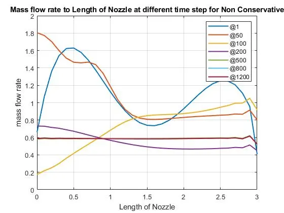
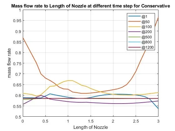
3. To plot variation of Mass flow rate distribution inside the nozzle at different time steps during the time-marching process.
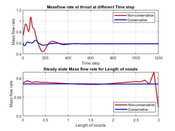
4. To Compare of Normalized mass flow rate distributions of both forms.

Theory: - While isentropic 1-D supersonic nozzle problem can be solved by analytical method, we are trying to get the same approximate result by using numerical method i.e., Mac-Cormack’s Method so as build the understanding of this method.

A nozzle is Convergent-Divergent tube used to control the characteristics of the flow such as velocity, pressure etc.

Governing equations:

we are assuming a 1-D flow i.e., properties changes with only x direction. There are 3 equation one for each Continuity, Momentum and Energy for each form (conservative and Non-Conservative).

These equations are follows:

Non-conservative:

1. Continuity: `(∂ρ^')/(∂t^' )=-ρ^' ((∂V^')/(∂x^' ))-ρ^' V^' (∂(lnA^' )/(∂x^' ))-V^' ((∂ρ^')/(∂x^' ))`
2. Momentum: `( ∂V^')/(∂t^' )=-V^' ((∂V^')/(∂x^' ))-(1/γ)((∂T^')/(∂x^' )+T^'/ρ^' ((∂ρ^')/(∂x^' )))`
3. Energy: `(∂T^')/(∂t^' )=-V^' ((∂T^')/(∂x^' ))-(γ-1)T'[(∂V^')/(∂x^' )+V^' ∂(lnA^' )/(∂x^' )]`

Non-conservative:

1. Continuity: `(∂(ρ^' A^' ))/(∂t^' )+(∂(ρ^' A^' V^'))/(∂x^' )=0`
2. Momentum: `(∂(ρ^' A^' V^' ))/(∂t^' )+(∂[ρ^' A^('V^'2 )+(1/γ) ρ^' A^' ])/(∂x^' )=(1/γ) ρ^' ((∂A^')/(∂x^' ))`
3. Energy: `(∂[ρ^' (e^'/(γ-1 )+(γ/2) V^'2 ) A^' ])/(∂t^' )+(∂[ρ^' (e^'/(γ-1)+(γ/2 ) V^'2 ) V^' A^'+ρ^' A^' V^' ])/(∂x^' )=0`

here the variables with dash denotes the ratio of properties to peak values hence non dimensional.

The conservative form is further simplified into solution vectors, Flux vector and source term.

For time step calculation: `dt= cfl* dx/(a+v)`

where cfl is taken 0.5 and a is square root of temperature for that grid and v is the local velocity of the grid. dt is calculated for every grid and minimum values is taken as time step.

Mac-Cormack’s Method: -

This method is explicit finite difference technique which is second order accurate in both space and time.

Let f(x) is the equation to be solved. Then the following steps are followed

1. Initial profile: Before the calculation, the initial profile for all the flow field variables which are velocity, density and temperature has to be determined. These are guessing values but should be specified with more awareness on the problem.

2. Predictor step: In this step Forward differencing is used to obtain derivatives `((∂f)/dt) _p=(f(i+1)-f(i))/(Δx )`

3. Solution update: `f_p=f_(Initial)+((∂f)/(∂t))_p⋅Δt`

fp = Flow field variables calculated after the predictor step

`f_(Initial)` = flow field variable in the initial step

Δt = time step size

4. Corrector step: `((∂f_p)/dt) _c=(f(i)-f(i-1))/(Δx )`

`((∂f)/dt)_(avg)=0.5(((∂f)/dt)_p+((∂f_p)/dt)_c)`

5. Final solution update: `f_(sol)=f_(Initial)+((∂f)/(∂t))_(avg)⋅Δt`

`f_(sol)` =Final solution of the flow field variables for the first-time step

MATLAB code: -

There is a Main program with 2 functions for conservative form and non-conservative form separately

Main Program:

clear all
close all
clc

%inputs
n=[31,61,91]; 

for k=1:3
l=3;
gamma=1.4;

nt=1200;
cfl=0.5;

%function calling
%for Non conservative
[mfr_nc,mfr_th_nc,table_initial_nc,table_final_nc]=OneD_Non_conservative(l,n(k),nt,cfl);
if k==1
    mfr_nc_31=mfr_nc;
    mfr_th_nc_31=mfr_th_nc;
    table_final_nc_31=table_final_nc;
elseif k==2
    mfr_nc_61=mfr_nc;
    mfr_th_nc_31=mfr_th_nc;
    table_final_nc_61=table_final_nc;
elseif k==3
    mfr_nc_91=mfr_nc;
    mfr_th_nc_31=mfr_th_nc;
    table_final_nc_91=table_final_nc;
end

[mfr_c,mfr_th_c,table_initial_c,table_final_c]=oneD_conservative(l,n(k),nt,cfl);

if k==1
    mfr_c_31=mfr_c;
    mfr_th_c_31=mfr_th_c;
    table_final_c_31=table_final_c;
elseif k==2
    mfr_c_61=mfr_c;
    mfr_th_c_31=mfr_th_c;
    table_final_c_61=table_final_c;
elseif k==3
    mfr_c_91=mfr_c;
    mfr_th_c_31=mfr_th_c;
    table_final_c_91=table_final_c;
end
end

x=linspace(0,l,n(k));

figure(7)
subplot(2,1,1)
plot(1:nt,mfr_th_nc,'r','linewidth',2);
hold on
plot(1:nt,mfr_th_c,'b','linewidth',2);
grid on 
xlabel('Time step');
ylabel('Mass flow rate');
title('Massflow rate at throat at different Time step');
legend('Non-conservative','Conservative');

subplot(2,1,2)
plot(x,mfr_nc,'r','linewidth',2);
hold on
plot(x,mfr_c,'b','linewidth',2);
xlabel('Length of nozzle');
ylabel('Mass flow rate');
title('Steady state Mass flow rate for Length of nozzle');
legend('Non-conservative','Conservative');
grid on 

Non- conservative:

function [mfr_nc,mfr_th_nc,table_initial_nc,table_final_nc]=OneD_Non_conservative(l,n,nt,cfl)

x=linspace(0,l,n);
dx=x(2)-x(1);
gamma=1.4;

% initial conditions
rho=1-0.3146.*x;
T=1-0.2314.*x;
v=(0.1+1.09.*x).*(T.^.5);
a=1+2.2.*(x-1.5).^2;
mach=v./T.^.5;
%mfr=rho.*a.*v;
p=rho.*T;

%initial primitive variables table
table_initial_nc=table(x',a',rho',v',T','VariableNames',{'distance','area','Density','velocity','Temperature'});

%time step calculation
for c=1:length(x)
dt_all(c)=cfl*(dx/((T(c))^.5 +v(c)));
end
dt=min(dt_all);

for i=1:nt
    rho_old=rho;
    T_old=T;
    v_old=v;
  for j=2:n-1
    %predictor step
   
     dvdx=(v(j+1)-v(j))/dx;
     drhodx=(rho(j+1)-rho(j))/dx;
     dTdx=(T(j+1)-T(j))/dx;
     dlnadx=(log(a(j+1))-log(a(j)))/dx;
     
     drhodt_p(j)= -rho(j)*dvdx -rho(j)*v(j)*dlnadx -v(j)*drhodx ;
     dvdt_p(j)= -v(j)*dvdx - (1/gamma)*(dTdx + (T(j)/rho(j))*drhodx);
     dTdt_p(j)= -v(j)*dTdx -(gamma-1)*T(j)*(dvdx + v(j)*dlnadx);
     
     %solution update
     v(j)=v_old(j) + dvdt_p(j)*dt;
     rho(j)=rho_old(j) + drhodt_p(j)*dt;
     T(j)=T_old(j) + dTdt_p(j)*dt;
     
        
  end
  
  for j=2:n-1
      %corrector step
   
     dvdx=(v(j)-v(j-1))/dx;
     drhodx=(rho(j)-rho(j-1))/dx;
     dTdx=(T(j)-T(j-1))/dx;
     dlnadx=(log(a(j))-log(a(j-1)))/dx;
     
     drhodt_c(j)= -rho(j)*dvdx -rho(j)*v(j)*dlnadx -v(j)*drhodx ;
     dvdt_c(j)= -v(j)*dvdx - (1/gamma)*(dTdx + (T(j)/rho(j))*drhodx);
     dTdt_c(j)= -v(j)*dTdx -(gamma-1)*T(j)*(dvdx + v(j)*dlnadx);
     
      
  end
  
   %calculating average
     
   drhodt=.5*(drhodt_p+drhodt_c);
   dvdt=.5*(dvdt_p+dvdt_c);
   dTdt=.5*(dTdt_p+dTdt_c);
   
   %final update
   
   for k=2:n-1
       rho(k)=rho_old(k)+ drhodt(k)*dt;
       v(k)=v_old(k)+ dvdt(k)*dt;
       T(k)=T_old(k)+ dTdt(k)*dt;
   end
   
   %boundary condition
   %inlet
   v(1)=2*v(2)-v(3);
   
   %outlet
   v(n)=2*v(n-1)-v(n-3);
   rho(n)=2*rho(n-1)-rho(n-3);
   T(n)=2*T(n-1)-T(n-3);
   
   mach=v./T.^.5;
   mfr_nc=rho.*a.*v;
   p=rho.*T;
  
  % throat value
  th=find(a==1);
  mfr_th_nc(i)=mfr_nc(th);
  rho_th_nc(i)=rho(th);
  v_th_nc(i)=v(th);
  p_th_nc(i)=p(th);
  mach_th_nc(i)=mach(th);
  T_th_nc(i)=T(th);
 
  %plotting primitive variables wrt length of nozzle
  figure(1)
  subplot(4,1,1)
  sgtitle('Primitive variables wrt length of nozzle');
  plot(x,p,'r','linewidth',2)
  ylabel('Pressure');
  title(sprintf('Time step: %d',i));
  grid on 
  pause(0.03)
  
  subplot(4,1,2)
  plot(x,T,'r','linewidth',2)
  ylabel('Temperature');
  grid on 
  pause(0.03)
  
  subplot(4,1,3)
  plot(x,rho,'r','linewidth',2)
  ylabel('Density');
  grid on
  pause(0.03)
  
  subplot(4,1,4)
  plot(x,mach,'r','linewidth',2)
  ylabel('Mach No.');
  xlabel('Length of Nozzle');
  grid on 
  pause(0.03)
 
  if (i==1)
   mfr1=mfr_nc;
elseif (i==50)
   mfr50=mfr_nc;
elseif (i==100)
   mfr100=mfr_nc;
elseif (i==200)
    mfr200=mfr_nc;
elseif (i==500)
    mfr500=mfr_nc;
elseif (i==800)
    mfr800=mfr_nc;
elseif (i==1200)
    mfr1200=mfr_nc;
  end
  
end

figure(2)
plot(x,mfr1,x,mfr50,x,mfr100,x,mfr200,x,mfr500,x,mfr800,x,mfr1200,'linewidth',1.5)
xlabel('Length of Nozzle');
ylabel('mass flow rate');
legend('@1','@50','@100','@200','@500','@800','@1200');
title('Mass flow rate to Length of Nozzle at different time step for Non Conservative');
grid on 

%plotting primitive variables wrt time steps
  
  figure(3)
  subplot(4,1,1)
  sgtitle('Primitive variables wrt Time steps at Throat');
  plot(1:nt,p_th_nc,'r','linewidth',2);
  ylabel('Pressure');
  ylim([0,1.1]);
  grid on 
  
  subplot(4,1,2)
  plot(1:nt,T_th_nc,'r','linewidth',2)
  ylabel('Temperature');
  ylim([0,1.1]);
  grid on 
  
  subplot(4,1,3)
  plot(1:nt,rho_th_nc,'r','linewidth',2)
  ylabel('Density');
  ylim([0,1.1]);
  grid on 
  
  subplot(4,1,4)
  plot(1:nt,mach_th_nc,'r','linewidth',2)
  ylabel('Mach No.');
  xlabel('Time step');
  ylim([0,4]);
  grid on 
%final primitive variables table
string={'distance','area','Density','velocity','Temperature','pressure','Mach'};
table_final_nc=table(x',a',rho',v',T',p',mach','VariableNames',string);
        
end

Conservative:

function [mfr_c,mfr_th_c,table_initial_c,table_final_c]=oneD_conservative(l,n,nt,cfl)

x=linspace(0,l,n);
dx=x(2)-x(1);
gamma=1.4;

% initial conditions
for i=1:length(x)
    if (x(i)<.5)
        rho(i)=1;  
        T(i)=1;
    elseif (x(i)>=0.5) && (x(i)<=1.5)
        rho(i)=1-0.366*(x(i)-.5);
        T(i)=1-0.167*(x(i)-.5);
    elseif (x(i)>1.5) && (x(i)<=3)
        rho(i)=0.634-0.3879*(x(i)-1.5);
        T(i)=0.833-0.3507*(x(i)-1.5);
    end
end
a=1+2.2.*(x-1.5).^2;

%solution vectors u1,u2and u3
u1=rho.*a;
u2=0.59*ones(1,length(x));
v=u2./u1;
u3=rho.*a.*((T/(gamma-1)) +((gamma/2)*v.^2));

mach=v./T.^.5;
mfr_c=u2;
p=rho.*T;

%initial primitive variables table
string1={'distance','area','Density','velocity','Temperature','U1','U2','U3'};
table_initial_c=table(x',a',rho',v',T',u1',u2',u3','VariableNames',string1);

%time step calculation
for c=1:length(x)
dt_all(c)=cfl*(dx/((T(c))^.5 +v(c)));  
end
dt=min(dt_all);

for t=1:nt
    
    u1_old=u1;
    u2_old=u2;
    u3_old=u3;
  
    %flux vectors
    f1=u2;
    f2=((u2.^2)./u1)+((gamma-1)/gamma)*(u3 -((gamma/2)*(u2.^2)./u1));
    f3=((gamma*u2.*u3)./u1)-((gamma*(gamma-1)/2)*(u2.^3)./(u1.^2));
    
    for j=2:n-1
        
    %source term
    j1(j)=(1/gamma)*rho(j)*T(j)*((a(j+1)-a(j))/dx);  
    
    %predictor step
    du1_dt_p(j)= -((f1(j+1)-f1(j))/dx);
    du2_dt_p(j)= -((f2(j+1)-f2(j))/dx) + j1(j);
    du3_dt_p(j)= -((f3(j+1)-f3(j))/dx);
    
    %solution updating
    u1(j)=u1_old(j) + du1_dt_p(j)*dt;
    u2(j)=u2_old(j) + du2_dt_p(j)*dt;
    u3(j)=u3_old(j) + du3_dt_p(j)*dt;
    
    end
    

    %primitives updating
    rho=u1./a;
    T=(gamma-1)*(u3./u1-((gamma/2)*(u2./u1).^2)); 
    
    %updating flux vectors
    f1=u2;
    f2=((u2.^2)./u1)+((gamma-1)/gamma)*(u3 -((gamma/2)*(u2.^2)./u1));
    f3=((gamma*u2.*u3)./u1) - ((gamma*(gamma-1)/2)*(u2.^3)./(u1.^2));
    
    for j=2:n-1
    %updating source term
    j2(j)=(1/gamma)*rho(j)*T(j)*((a(j)-a(j-1))/dx);
    
        
    %corrector step
    du1_dt_c(j)= -((f1(j)-f1(j-1))/dx);
    du2_dt_c(j)= -((f2(j)-f2(j-1))/dx) + j2(j);
    du3_dt_c(j)= -((f3(j)-f3(j-1))/dx);
    
    end
    
    %average of steps
    du1_dt=0.5*(du1_dt_p + du1_dt_c);
    du2_dt=0.5*(du2_dt_p + du2_dt_c);
    du3_dt=0.5*(du3_dt_p + du3_dt_c);
    
for j=2:n-1
    
    %final update
    u1(j)= u1_old(j) + du1_dt(j)*dt;
    u2(j)= u2_old(j) + du2_dt(j)*dt;
    u3(j)= u3_old(j) + du3_dt(j)*dt;
end

   %boundary conditions
   %Entry
   u1(1)=rho(1)*a(1);
   u2(1)=2*u2(2)-u2(3);
   v(1)=u2(1)/u1(1);
   u3(1)=rho(1)*a(1)*((T(1)/(gamma-1))+((gamma/2)*v(1)^2));
   
   %Exit
   u1(n)=2*u1(n-1)-u1(n-2);
   u2(n)=2*u2(n-1)-u2(n-2);
   u3(n)=2*u3(n-1)-u3(n-2);
    
 %calcultinf final primitive 
 rho=u1./a;
 v=u2./u1;
 T=(gamma-1).*(u3./u1-(gamma/2).*(u2./u1).^2); 
 mach=v./T.^.5;
 mfr_c=u2;
 p=rho.*T;
 
 % calculating throat value
  th=find(a==1);
  mfr_th_c(t)=mfr_c(th);
  rho_th_c(t)=rho(th);
  v_th_c(t)=v(th);
  p_th_c(t)=p(th);
  mach_th_c(t)=mach(th);
  T_th_c(t)=T(th);
  
   


 %plotting primitive variables wrt length of nozzle
  figure(4)
  subplot(4,1,1)
  sgtitle('Primitive variables wrt length of nozzle');
  plot(x,p,'linewidth',2)
  ylabel('Pressure');
  title(sprintf('Time step: %d',t));
  pause(0.03)
  grid on 
  
  subplot(4,1,2)
  plot(x,T,'linewidth',2)
  ylabel('Temperature');
  pause(0.03)
  grid on 
  
  subplot(4,1,3)
  plot(x,rho,'linewidth',2)
  ylabel('Density');
  pause(0.03)
  grid on 
  
  subplot(4,1,4)
  plot(x,mach,'linewidth',2)
  ylabel('Mach No.');
  xlabel('Length of Nozzle');
  pause(0.03)
  grid on 
  
 if (t==1)
   mfr1=mfr_c;
elseif (t==50)
   mfr50=mfr_c;
elseif (t==100)
   mfr100=mfr_c;
elseif (t==200)
    mfr200=mfr_c;
elseif (t==500)
    mfr500=mfr_c;
elseif (t==800)
    mfr800=mfr_c;
elseif (t==1200)
    mfr1200=mfr_c;
  end
 
 

end

 figure(5)
plot(x,mfr1,x,mfr50,x,mfr100,x,mfr200,x,mfr500,x,mfr800,x,mfr1200,'linewidth',1.5)
xlabel('Length of Nozzle');
ylabel('mass flow rate');
legend('@1','@50','@100','@200','@500','@800','@1200');
title('Mass flow rate to Length of Nozzle at different time step for Conservative');
grid on  
 %plotting primitive variables wrt time steps
  
  figure(6)
  subplot(4,1,1)
  sgtitle('Primitive variables wrt Time steps at Throat');
  plot(1:nt,p_th_c,'linewidth',2)
  ylabel('Pressure');
  ylim([0,1.1]);
  grid on 
  
  subplot(4,1,2)
  plot(1:nt,T_th_c,'linewidth',2)
  ylabel('Temperature');
  ylim([0,1.1]);
  grid on 
  
  subplot(4,1,3)
  plot(1:nt,rho_th_c,'linewidth',2)
  ylabel('Density');
  ylim([0,1.1]);
  grid on 
  
  subplot(4,1,4)
  plot(1:nt,mach_th_c,'linewidth',2)
  ylabel('Mach No.');
  xlabel('Time step');
  ylim([0,4]);
  grid on 
  
%final primitive variables table
string={'distance','area','Density','velocity','Temperature','pressure','Mach','U1','U2','U3'};
table_final_c=table(x',a',rho',v',T',p',mach',u1',u2',u3','VariableNames',string);
end

Results: - All the plot are for grid no. 31

1. Non- conservative form

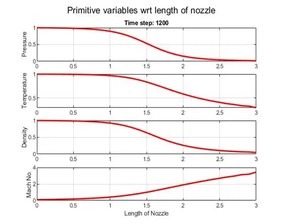
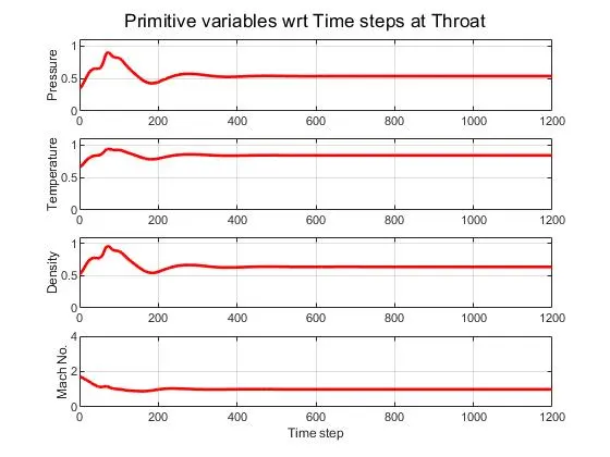
2. For Conservative form

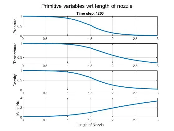
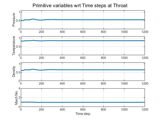
3. Mass flow rate at different time step

4. Comparison between Mass flow rates for conservative and non-conservative form

Grid Independence test:

It is done to check the accuracy of the value for certain number of grids, and find the best number of grids to get the most accurate values.

The values in below table ar at throat region and taken from the tables formed in the codes and are ratio to the value at inlet.

PRIMITIVES	EXACT VALUE	GRID NO. = 31		GRID NO. = 61		GRID NO. = 91
		CONSERVATIVE	NON-CONSERVATIVE	CONSERVATIVE	NON-CONSERVATIVE	CONSERVATIVE	NON-CONSERVATIVE
Density	.634	.6529	.6389	.6389	.6367	.6359	.6295
Temperature	.833	.8413	.8365	.8354	.8349	.8341	.8312
pressure	.528	.5492	.5342	.5337	.5316	.5304	.5233
Mach No.	1	.9711	.999	.9978	1	.9992	1

Conclusion:

1. The plot of conservative forms is smoother and have less fluctuation as compared to the Non conservative form.
2. the mass flow rates at less no. of time steps have more fluctuation in Non-conservative as initial values are assumed to be equal to the values at reservoir which is not the case at inlet, hence more accurate initial condition can reduce.
3. In grid independence test we can observe the primitive values for Non conservative form are closer to exact value then the Conservative, since Non conservative value provides better results for primitive values and Conservative provides better values for Flux variables.
4. As there is insignificant change in values as grid no. are doubled or tripled, we have to keep in mind as these increase the calculation time, hence grid size should be chosen which gives balanced results with appropriate execution time.