Week 7 - Simulation of a 1D Super-sonic nozzle flow simulation using Macormack Method
OBJECTIVE:
- To write a matlab program for the quasi 1D supersonic nozzle flow simulation for both conservative and non conservative form of governing equation using maccormack method.
- To compare the result obtained by conservative and non conservative form of governing equation.
- To perform a grid dependence test on the solution.
MACCORMACK METHOD:
In CFD, the maccormack method is widely used discretization scheme for the numerical solution of hyperbolic partial differential equations.
This method is used which provides 2nd order accuracy without the involvement of 2nd derivative, thus reducing the complexity of the mathematical calculation.
The MacCormack method is well suited for non linear equations (Inviscid Burger's equation, Euler's equation, etc.) The order of differencing can be reversed for the time step (i.e., forward/backward followed by backward/forward).
For nonlinear equations, this procedure provides the best results.
For linear equations, the MacCormack scheme is equivalent to the Lax wendroff method.
STEPS IN MACCORMACK TECHNIQUE:
- Predictor step
- Corrector step
- Average time step
- Final solution update
PREDICTOR STEP:
We are having our conservative and non conservative form of 1D supersonic nozzle flow. We have to use the forward differencing for the spatial derivatives. And we need to do the solution update for the flow field variables.
CORRECTOR STEP:
In the corrector step the spatial derivatives are discretized by using backward differencing.
AVERAGE TIME STEP:
The average time step is calculated by averaging the predictor step and corrector step.
`((delrho)/(delt))_(avg) = 0.5*[((delrho)/(delt))^i+((delrho)/(delt))_i^(t+trianglet)]`
The final solution is updated by using the average time step,
`(rho_i^(t+trianglet)) = rho_i^t + ((delrho)/(delt))*(trianglet)_(avg)`
- CONSERVATIVE FORM:
The equations obtained from the finite control volume fixed in space in either integral or PDE form are called the conservation form of the governing equation.
- NON-CONSERVATION FORM:
The equations obtained from the finite control volume moving with fluid in either integral or PDE equations are called the non-conservation form of governing equation.
1D SUPERSONIC FLOW NOZZLE:
When mach number is greater than 1 then this condition is known as supersonic condition i.e., velocity faster than sound. mach number generally represents the speed of aircraft and missile with respect to sound.
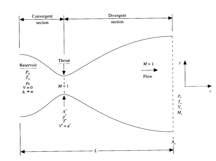
We consider a steady, isentropic flow through a convergent-divergent nozzle as shown above. the flow at the inlet to the nozzle comes from the reservoir where the pressure and temperature are p0 and t0 respectively these are the stagnation values. the cross sectional area of the reservoir is large and hence the velocity is very small. The flow expands isentropically to supersonic speeds at the nozzle exit, where pe, te, ve and me are exit pressure, temperature, velocity and mach number respectively.
The flow is locally subsonic in the convergent section, sonic at the throat and supersonic at divergent section of the nozzle.
The sonic flow (mach=1) at the throat means that the local velocity at this location is equal to the local speed of sound. The pressure, temperature, velocity and area are p*, t*, v* and a* respectively.
We make the assumption that the flow properties vary only with x; tantamount to assuming uniform flow properties across any given cross section. Such flow is defined as quasi one dimensional flow.
INITIAL CONDITION AND NOZZLE SHAPE:
NON-CONSERVATIVE FORM:
GOVERNING EQUATION:
CONTINUITY EQUATION:
`(delrho)/(delt) = -rho*((delv)/(delx)) – rho*v*(lna/(delx)) – v*((delrho)/(delx))`
MOMENTUM EQUATION:
`(delv)/(delt) = -v*((delv)/(delx))-((1/gamma)*((delt)/(delx)+(t/rho)*((delt)/(delx))))`
ENERGY EQUATION:
`(delt)/(delt) = -v*((delt)/(delx))-((gamma-1)*t*[(delv)/(delx)+v*((lna)/(delx))])`
INITIAL CONDITION at t=0,
Area, a = 1+2.2(x-1.5)^2 0 <= x <= 3
Density, rho = 1-0.3146*x
Temperature, t = 1- 0.2314*x
Velocity, v = (0.1+1.09*x)*(t^0.5)
Pressure, p = rho*t
Mach number, m = v/t^0.5
BOUNDARY CONDITIONS:
Inlet, v(1) = 2*v(2) – v(3)
Outlet, v(n) = 2*v(n-1) – v(n-2)
p(n) = 2*p(n-1) – p(n-2)
t(n) = 2*t(n-1) – t(n-2)
TIMESTEP CALCULATION:
`Deltat = c*((Deltax)/(t^0.5+v))`
Where, deltat = time step,
c = courant number
a = local velocity of sound a = t^0.5
v = velocity.
CONSERVATIVE FORM:
SOLUTION VECTOR:
`u1 = rho*a`
`u2 = rho*a*v`
`u3 = rho*a*((t/(gamma-1))+((gamma/2)*v^2))`
GOVERNING EQUATION:
FLUX TERMS:
`f1 = u_2`
`f2 = ((u_2^2)/u_1)+(((gamma-1)/gamma)*(u_3-((gamma/2)*((u_2^2)/u_1))))`
`f3 = ((gamma*(u_2*u_3)/u_1)-(((gamma*(gamma-1))/2)*(u_2^3)/(u_1^2))`
SOURCE TERMS:
`J2 = (1/gamma)*rho*(dela)/(delx)`
CONTINUITIY EQUATION:
`(delu_1)/(delt) = -(delf1)/(delx)`
MOMENTUM EQUATION:
`(delu_2)/(delt) = -(delf2)/(delx)+j2`
ENERGY EQUATION:
`(delu_3)/(delt) = -(delf3)/(delx)`
INITIAL CONDITION:
For 0 <= x <= 0.5, rho = 1, t=1
For 0.5 <= x <= 1.5, rho = 1 – 0.366*(x-0.5)
T = 1 – 0.167*(x-0.5)
For 1.5 <= x <= 3.5, rho = 0.634 – 0.3879*(x-1.5)
T = 0.833 – 0.3507*(x-1.5)
Pressure, p = rho*t
Mach number, M = v/t^0.5
V = u2 = 0.59/rho*a
BOUNDARY CONDITIONS:
INLET:
u2(1) = 2*u2(2)-u2(3)
OUTLET:
u1(n) = 2*u1(n-1)-u1(n-2)
u2(n) = 2*u2(n-1)-u2(n-2)
u3(n) = 2*u3(n-1)-u3(n-2)
MATLAB CODE:
MAIN CODE:
clear all
close all
clc

%inputs
n = 31;
x = linspace(0,3,n);

%grid spacing
dx = x(2)-x(1);

%gamma
gamma = 1.4;

%courant number
c = 0.5;

%area
a = 1+(2.2*(x-1.5).^2);

%time step
nt = 1400;

%throat point
throat = ((n-1)/2)+1;

%function calling
%non conservative
tic
[rho,t,v,p,mach,mass_flow,rho_t,t_t,v_t,p_t,mach_t,mass_flow_t,rho_res,t_res,v_res] = non_conservative(x,dx,n,a,c,gamma,nt,throat);
non_conservative_time = toc;

%conservative
tic
[rho_c,t_c,v_c,p_c,mach_c,mass_flow_c,rho_t_c,t_t_c,v_t_c,p_t_c,mach_t_c,mass_flow_t_c,rho_res_c,t_res_c,v_res_c] = conservative(x,dx,n,a,c,gamma,nt,throat);
conservative_time = toc;

%plotting
figure(3)
subplot(4,1,1)
plot(x,rho,'r',x,rho_c,'b*')
xlabel('length of the nozzle')
ylabel('density ratio')
title('density profile')
legend('non conservative','conservative','location','southwest')

subplot(4,1,2)
plot(x,p,'r',x,p_c,'b*')
xlabel('length of the nozzle')
ylabel('pressure ratio')
title('pressure profile')
legend('non conservative','conservative','location','southwest')

subplot(4,1,3)
plot(x,t,'r',x,t_c,'b*')
xlabel('length of the nozzle')
ylabel('temperature ratio')
title('temperature profile')
legend('non conservative','conservative','location','southwest')

subplot(4,1,4)
plot(x,mach,'r',x,mach_c,'b*')
xlabel('length of the nozzle')
ylabel('mach number')
title('mach number profile')
legend('non conservative','conservative','location','northwest')

figure(4)
subplot(3,2,1)
plot(1:nt,rho_t,'r',1:nt,rho_t_c,'k')
xlabel('time step')
ylabel('density')
title('density profile')
legend('non conservative','conservative')

subplot(3,2,2)
plot(1:nt,p_t,'r',1:nt,p_t_c,'k')
xlabel('time step')
ylabel('pressure')
title('pressure profile')
legend('non conservative','conservative')

subplot(3,2,3)
plot(1:nt,t_t,'r',1:nt,t_t_c,'k')
xlabel('time step')
ylabel('temperature')
title('temperature profile')
legend('non conservative','conservative','location','southeast')

subplot(3,2,4)
plot(1:nt,v_t,'r',1:nt,v_t_c,'k')
xlabel('time step')
ylabel('velocity')
title('velocity profile')
legend('non conservative','conservative')

subplot(3,2,5)
plot(1:nt,mach_t,'r',1:nt,mach_t_c,'k')
xlabel('time step')
ylabel('mach number')
title('mach number profile')
legend('non conservative','conservative')

subplot(3,2,6)
plot(1:nt,mass_flow_t,'r',1:nt,mass_flow_t_c,'k')
xlabel('time step')
ylabel('mass flow rate')
title('mass flow rate profile')
legend('non conservative','conservative')

figure(5)
plot(x,rho,'g',x,mach,'r')
grid on
xlabel('length of the nozzle')
ylabel('y axis')
title('length vs density and mach number')
legend('density','mach number','location','northwest')

figure(6)
plot(x,mass_flow,'r',x,mass_flow_c,'b')
grid on
xlabel('length of the nozzle')
ylabel('mass flow rate')
title('length vs mass flow rate')
legend('non conservative','conservative','location','northwest')

figure(7)
plot(1:nt,rho_res,'r',1:nt,t_res,'b',1:nt,v_res,'g')
grid on
xlabel('time step')
ylabel('density,temperature,velocity')
title('residual convergence-non conservative flow')
legend('density','temperature','velocity')

figure(8)
plot(1:nt,rho_res_c,'r',1:nt,t_res_c,'b',1:nt,v_res_c,'g')
grid on
xlabel('time step')
ylabel('density,temperature,velocity')
title('residual convergence-conservative flow')
legend('density','temperature','velocity')
FUNCTION CODE:
CONSERVATIVE FORM:
function [rho,t,v,p,mach,mass_flow,rho_t,t_t,v_t,p_t,mach_t,mass_flow_t,rho_res_c,t_res_c,v_res_c] = conservative(x,dx,n,a,c,gamma,nt,throat)

%initial profile
for i = 1:n
    if (x(i) >= 0 && x(i) <= 0.5)
        rho(i) = 1;
        t(i) = 1;
    elseif (x(i) >= 0.5 && x(i) <= 1.5)
           rho(i) = (1-0.366*(x(i)-0.5));
           t(i) = (1-0.167*(x(i)-0.5));
    elseif (x(i) >= 1.5 && x(i) <= 3.5)
           rho(i) = 0.634-0.3879*(x(i)-1.5);
           t(i) = 0.833-0.3507*(x(i)-1.5);
    end
end

 %velocity
 v = 0.59./(rho.*a);

 %pressure
 p = rho.*t;

 %u1,u2,u3
 u1 = rho.*a;
 u2 = rho.*a.*v;
 u3 = rho.*a.*((t./(gamma-1))+((gamma/2).*(v.^2)));

 %time step
 dt = min(c.*(dx./((t.^0.5)+v)));

%outer time loop
for q = 1:nt

    %creating a copy
    u1_old = u1;
    u2_old = u2;
    u3_old = u3;

    %flux vector
    f1 = u2;
    f2 = ((u2.^2)./u1)+(((gamma-1)/gamma)*(u3-((gamma/2)*((u2.^2)./u1))));
    f3 = ((gamma*u2.*u3)./u1)-(gamma*(gamma-1)*(u2.^3))./(2*u1.^2);

    %predictor method
    for j = 2:n-1
        %continuity equation
        du1dt_p(j) = -(f1(j+1)-f1(j))/dx;

        %momentum equation
        j2(j)  = (1/gamma)*(rho(j)*t(j))*((a(j+1)-a(j))/dx);
        du2dt_P(j) = -((f2(j+1)-f2(j))/dx)+j2(j);

        %energy equation
        du3dt_p(j) = -(f3(j+1)-f3(j))/dx;

        %first solution update
        u1(j) = u1(j)+du1dt_p(j)*dt;
        u2(j) = u2(j)+du2dt_P(j)*dt;
        u3(j) = u3(j)+du3dt_p(j)*dt;
    end

    %updating flux vectors and variables
    rho = u1./a;
    v = u2./u1;
    t = (gamma-1)*((u3./u1)-((gamma*v.^2)/2));

    f1 = u2;
    f2 = ((u2.^2)./u1)+(((gamma-1)/gamma)*(u3-((gamma/2)*((u2.^2)./u1))));
    f3 = ((gamma*u2.*u3)./u1)-(gamma*(gamma-1)*(u2.^3))./(2*u1.^2);

    %corrector method
    for j = 2:n-1
        %continuity equation
        du1dt_c(j) = -(f1(j)-f1(j-1))/dx;

        %momentum equation
        j2(j)  = (1/gamma)*(rho(j)*t(j))*((a(j)-a(j-1))/dx);
        du2dt_c(j) = -((f2(j)-f2(j-1))/dx)+j2(j);

        %energy equation
        du3dt_c(j) = -(f3(j)-f3(j-1))/dx;
    end

    %compute the average time derivative
    du1dt = 0.5*(du1dt_p+du1dt_c);
    du2dt = 0.5*(du2dt_P+du2dt_c);
    du3dt = 0.5*(du3dt_p+du3dt_c);

    %final solution update
    for k = 2:n-1
        u1(k) = u1_old(k)+du1dt(k)*dt;
        u2(k) = u2_old(k)+du2dt(k)*dt;
        u3(k) = u3_old(k)+du3dt(k)*dt;
    end

    %apply the boundary conditions
    %inlet
    u2(1) = 2*u2(2)-u2(3);

    %outlet
    u1(n) = 2*u1(n-1)-u1(n-2);
    u2(n) = 2*u2(n-1)-u2(n-2);
    u3(n) = 2*u3(n-1)-u3(n-2);

    %update
    %density
    rho = u1./a;

    %velocity
    v = u2./u1;

    %temperature
    t = (gamma-1)*((u3./u1)-((gamma*v.^2)/2));

    %mass flow rate
    mass_flow = rho.*a.*v;

    %pressure
    p = rho.*t;

    %mach no
    mach = v./(t.^0.5);

    %calculation of quantities at throat
    rho_t(q) = rho(throat);
    t_t(q) = t(throat);
    v_t(q) = v(throat);
    p_t(q) = p(throat);
    mach_t(q) = mach(throat);
    mass_flow_t(q) = mass_flow(throat);

    %residual convergence
    rho_res_c(q) = du1dt(throat);
    t_res_c(q) = du2dt(throat);
    v_res_c(q) = du3dt(throat);

    %plotting
    figure(2)
    hold on
    if q == 50
       plot(x,mass_flow,'b','linewidth',2);
    else if q == 100
            plot(x,mass_flow,'g','linewidth',2);
        else if q == 150
             plot(x,mass_flow,'m','linewidth',2);
            else if q == 200
                 plot(x,mass_flow,'r','linewidth',2);
                else if q == 700
                     plot(x,mass_flow,'k','linewidth',2);
                     axis([0 3 0 1])
                     legend('50deltat','100deltat','150deltat','200deltat','700deltat','location','southeast');
                     xlabel('length of nozzle')
                     ylabel('mass flow rate')
                     title('variation of mass flow rate at different time step')
                     grid on
                     grid minor
                     end
                end
             end
         end
    end
end
end
NON-CONSERVATIVE FORM:
function [rho,t,v,p,mach,mass_flow,rho_t,t_t,v_t,p_t,mach_t,mass_flow_t,rho_res,t_res,v_res] = non_conservative(x,dx,n,a,c,gamma,nt,throat)

%initial profile
%density
rho = 1-(0.3146*x);
%temperature
t = 1-(0.2314*x);
%volume
v = (0.1+(1.09*x)).*t.^0.5;

%time step
dt = min(c*(dx./(t.^0.5+v)));

%outer time loop
for q = 1:nt

    %creating a copy
    rho_old = rho;
    v_old = v;
    t_old = t;

    %predictor method
    for j = 2:n-1
        dvdx = (v(j+1)-v(j))/dx;
        drhodx = (rho(j+1)-rho(j))/dx;
        dlogadx = (log(a(j+1))-log(a(j)))/dx;
        dtdx = (t(j+1)-t(j))/dx;

        %continuitiy equation
        drhodt_p(j) = -rho(j)*dvdx-rho(j)*v(j)*dlogadx-v(j)*drhodx;

        %momentum equation
        dvdt_p(j) = -v(j)*dvdx-((1/gamma)*(dtdx+((t(j)/rho(j))*drhodx)));

        %energy equation
        dtdt_p(j) = -v(j)*dtdx-((gamma-1)*t(j)*(dvdx+(v(j)*dlogadx)));

        %first solution update
        v(j) = v(j)+dvdt_p(j)*dt;
        rho(j) = rho(j)+drhodt_p(j)*dt;
        t(j) = t(j)+dtdt_p(j)*dt;
    end

    %corrector method
    for j = 2:n-1
        dvdx = (v(j)-v(j-1))/dx;
        drhodx = (rho(j)-rho(j-1))/dx;
        dlogadx = (log(a(j))-log(a(j-1)))/dx;
        dtdx = (t(j)-t(j-1))/dx;

        %continuitiy equation
        drhodt_c(j) = -rho(j)*dvdx-rho(j)*v(j)*dlogadx-v(j)*drhodx;

        %momentum equation
        dvdt_c(j) = -v(j)*dvdx-((1/gamma)*(dtdx+((t(j)/rho(j))*drhodx)));

        %energy equation
        dtdt_c(j) = -v(j)*dtdx-((gamma-1)*t(j)*(dvdx+(v(j)*dlogadx)));

    end

    %compute the average time derivative
    drhodt = 0.5*(drhodt_p+drhodt_c);
    dvdt = 0.5*(dvdt_p+dvdt_c);
    dtdt = 0.5*(dtdt_p+dtdt_c);

    %final solution update
    for k = 2:n-1
        rho(k) = rho_old(k)+drhodt(k)*dt;
        v(k) = v_old(k)+dvdt(k)*dt;
        t(k) = t_old(k)+dtdt(k)*dt;
    end

    %apply the boundary conditions
    %inlet
    v(1) = 2*v(2)-v(3);
    rho(1) = 1;
    t(1) = 1;

    %outlet
    v(n) = 2*v(n-1)-v(n-2);
    rho(n) = 2*rho(n-1)-rho(n-2);
    t(n) = 2*t(n-1)-t(n-2);

    %mass flow rate
    mass_flow = rho.*a.*v;

    %pressure
    p = rho.*t;

    %mach no
    mach = v./(t.^0.5);

    %calculation of quantities at throat
    rho_t(q) = rho(throat);
    t_t(q) = t(throat);
    v_t(q) = v(throat);
    p_t(q) = p(throat);
    mach_t(q) = mach(throat);
    mass_flow_t(q) = mass_flow(throat);

    %residual convergence
    rho_res(q) = drhodt(throat);
    t_res(q) = dtdt(throat);
    v_res(q) = dvdt(throat);

    %plotting
    figure(1)
    hold on
    if q == 50
       plot(x,mass_flow,'b','linewidth',2);
    else if q == 100
            plot(x,mass_flow,'g','linewidth',2);
        else if q == 150
             plot(x,mass_flow,'m','linewidth',2);
            else if q == 200
                 plot(x,mass_flow,'r','linewidth',2);
                else if q == 700
                     plot(x,mass_flow,'k','linewidth',2);
                     axis([0 3 0 2])
                     legend('50deltat','100deltat','150deltat','200deltat','700deltat');
                     xlabel('length of nozzle')
                     ylabel('mass flow rate')
                     title('variation of mass flow rate at different time step')
                     grid on
                     grid minor
                     end
                end
             end
         end
    end
end
end
OUTPUT:
TIME TAKEN:
FOR N = 31
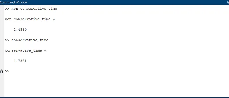
FOR N = 61:
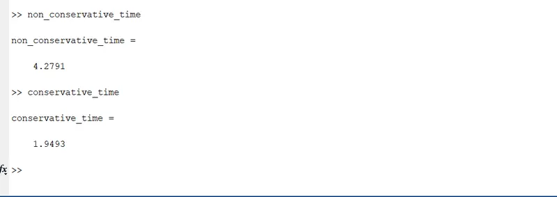
From the above figure, we can see that the non-conservative form takes more time than the conservative form.
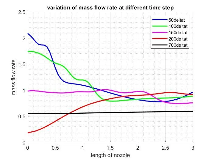
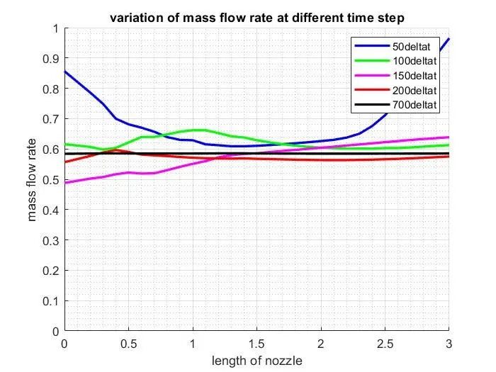
NON-DIMENSIONAL MASS FLOW RATE BEHAVIOUR ALONG NON-DIMENSIONAL LENGTH OF THE NOZZLE:
NON-CONSERVATIVE:
N = 31
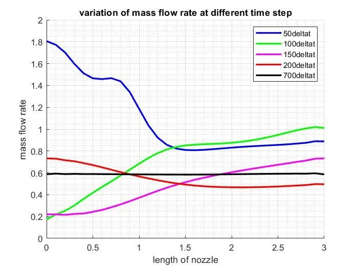
N= 61
CONSERVATIVE:
N =31
N =61
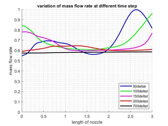
From the above plots, we can see that the mass flow distribution through the nozzle vary a lot in both forms. However in conservative solution the variation tends towards the steady state abit more than non-conservative approach. The point to note here is the initial conditions are different.
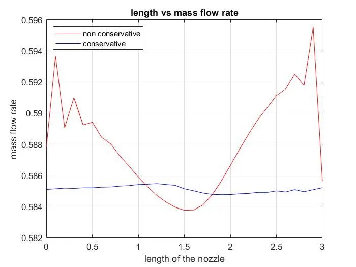
COMPARISON OF MASS FLOW RATE OF NON-CONSERVATIVE AND CONSERVATIVE FORM:
N = 31
N = 61
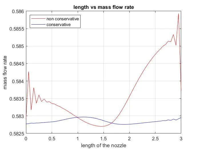
Mass flow solution of both forms are close to the analytical solution 0.579. the conservation form does a good job in preserving mass throughout the flow field because mass flow is a primary result. Whereas in non-conservation form the mass flow is obtained as secondary results.
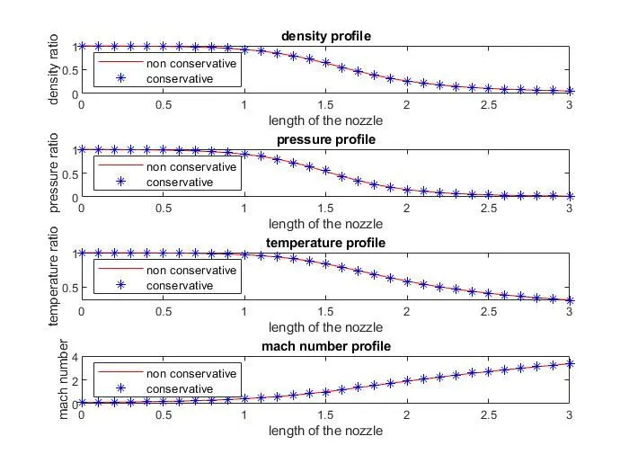
FLOW THROUGHOUT THE NOZZLE:
N = 31
N = 61
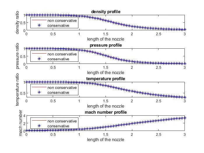
From the above plots, while comparing different flow properties with respect to length of the nozzle both the convergence and non- convergence form produces similar plots.
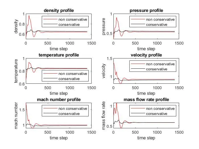
TIME VARIATION OF FLOW PARAMETERS ALONG THE NON-DIMENSIONAL LENGTH OF THE NOZZLE:
N = 31
N = 61
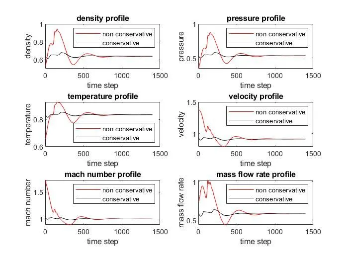
From the plots, we can say that the variation takes place at the earlier stages and after that steady state value is approached. at the earlier stages the flow field variables are driven by stronger potential and hence changes rapidly. At later times, as the steady state is approached it becomes more relaxed and the changes becomes much more smaller with time.
VARIATION OF DENSITY AND MACH NUMBER ALONG LENGTH OF THE NOZZLE:
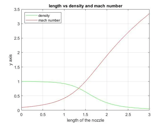
From the above plot, we can infer that density decreases with respect to length of the nozzle and mach number increases with respect to length of the nozzle.
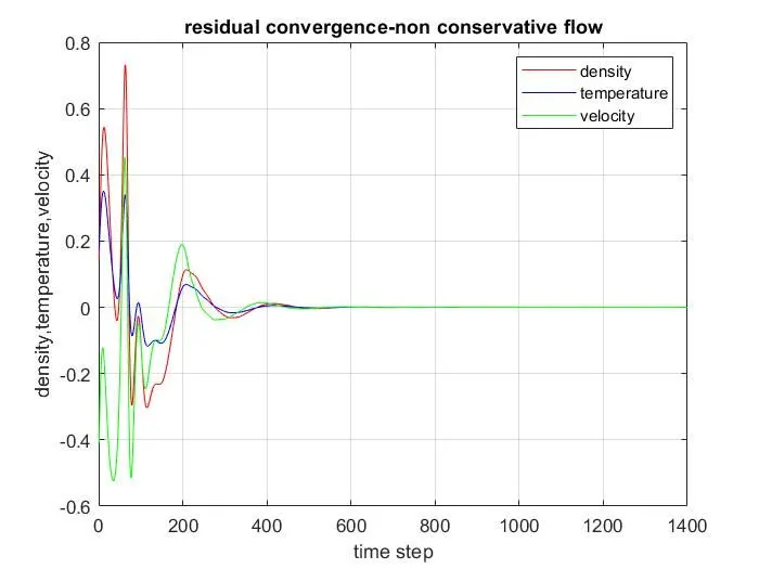
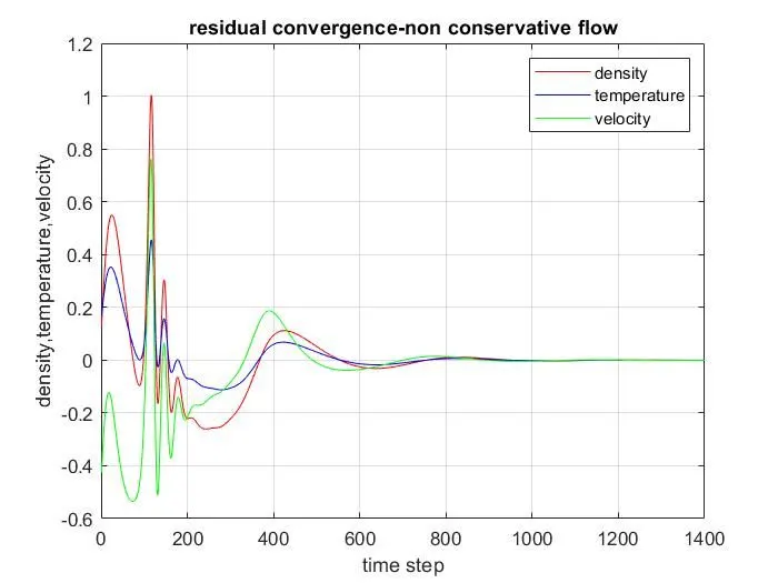
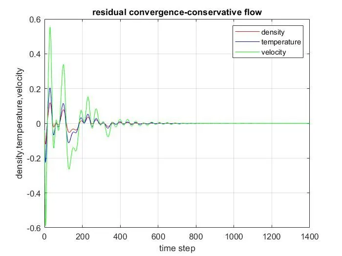
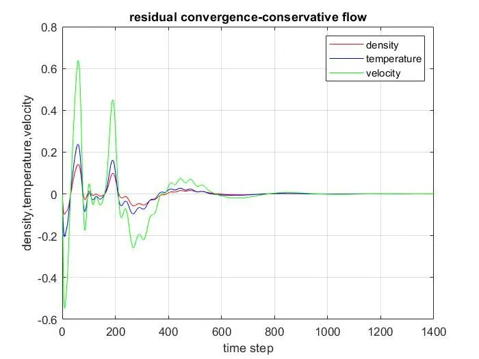
RESIDUAL CONVERGENCE:
NON-CONSERVATIVE:
N = 31
N = 61
CONSERVATIVE:
N = 31
N = 61
GRID DEPENDENCE TEST:
| GRID POINTS | EXACT | CONSERVATIVE | NON-CONSERVATIVE | |
| N = 31 | Pressure | 0.528 | 0.549 | 0.534 |
| Temperature | 0.833 | 0.841 | 0.837 | |
| Density | 0.634 | 0.652 | 0.639 | |
| N = 61 | Pressure | 0.528 | 0.534 | 0.533 |
| Temperature | 0.833 | 0.836 | 0.835 | |
| Density | 0.634 | 0.639 | 0.638 |
CONCLUSION:
1. The conservation form yields a better mass flow distribution and does a good job of conserving mass.
2. The non-conservation form leads to small residual.
3. The conservative method takes lesser time than non-conservative.
4. The non-conservative method have more accurate results with exact values than conservative.