Project 1 - Parsing NASA thermodynamic data

AIM:

• To write a function that extracts the 14 co-efficients and calculates the enthalpy, entropy, specific heats for all the species in the data file.
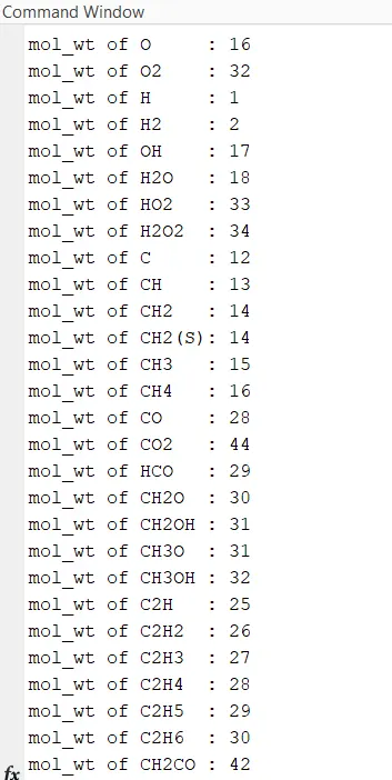
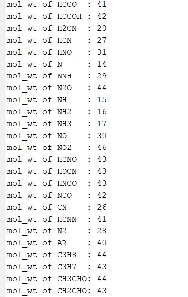
• To calculate the molecular weight of each species and display it in the command window.
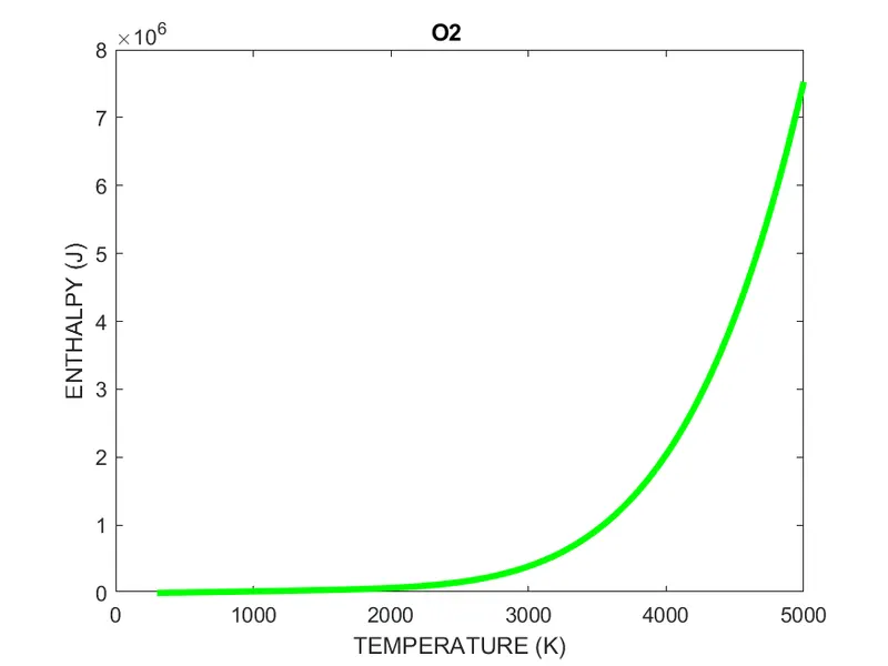
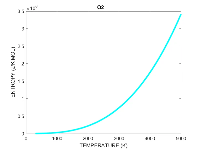
• To plot the cp, enthalpy and entropy for the local temperature range specific for each species.
• To save plots as images with appropriate names in separate folders for each species with suitable name.

THEORY:

               NASA came up with polynomials that can be used to evaluate thermodynamic properties such as cp, h, s. They have also documented the co-efficients that are required to evaluate these polynomials for 1000+ species.

               In this project, the THERMO.dat file is used for file parsing of thermodynamic files. The file contains species name, temperature ranges for individual species.

The formula used is shown below,

         Where,

                              Cp = specific heat (j/(kg k)),

                              H = enthalpy (j),

                              S = entropy (j/(k mol)),

                              R = universal gas constant (j/(k mol)),

                              T = temperature (k).

The first 7 co-efficients are high temperature co-efficients and the second 7 co-efficients are low temperature co-efficients.

MATLAB CODE:

MAIN MATLAB CODE:

clear all
close all
clc

f1=fopen('THERMO.dat','r');     %reading the file
line1=fgetl(f1);                %getting the first line
line2=fgetl(f1);                %getting the second line

split=strsplit(line2,' ');
split(1)=[];

low_temp=str2num(split{1});
mid_temp=str2num(split{2});
high_temp=str2num(split{3});

line3=fgetl(f1);
line4=fgetl(f1);
line5=fgetl(f1);

%for calculating species
%for loop for total co_efficients
for i=1:53
    %extracting speciesname
    species=fgetl(f1);
    species_name=species(1:6);
    
    %extracting coefficients from line7,
    line7=fgetl(f1);
    line8=fgetl(f1);
    line9=fgetl(f1);

    %finding string'E'
    b=findstr(line7,'E');
    c=findstr(line8,'E');
    d=findstr(line9,'E');

    %individual coefficients
    %line7
    a1=line7(1:b(1)+3);
    a1=str2num(a1);

    a2=line7(b(1)+4:b(2)+3);
    a2=str2num(a2);

    a3=line7(b(2)+4:b(3)+3);
    a3=str2num(a3);

    a4=line7(b(3)+4:b(4)+3);
    a4=str2num(a4);

    a5=line7(b(4)+4:b(5)+3);
    a5=str2num(a5);

    %line8
    a6=line8(1:c(1)+3);
    a6=str2num(a6);

    a7=line8(c(1)+4:c(2)+3);
    a7=str2num(a7);

    a8=line8(c(2)+4:c(3)+3);
    a8=str2num(a8);

    a9=line8(c(3)+4:c(4)+3);
    a9=str2num(a9);

    a10=line8(c(4)+4:c(5)+3);
    a10=str2num(a10);

    %line9
    a11=line9(1:d(1)+3);
    a11=str2num(a11);

    a12=line9(d(1)+4:d(2)+3);
    a12=str2num(a12);

    a13=line9(d(2)+4:d(3)+3);
    a13=str2num(a13);

    a14=line9(d(3)+4:d(4)+3);
    a14=str2num(a14);
    
    %creating the folder'species'to save the plots
    mkdir(['D:\NIRMAL\skill lync\workspace\nasa\species\',species_name]);
    r=8.314;
    t=linspace(low_temp,high_temp,500);
    
    %calling the function
    c_p = r*specific_heat(a1,a2,a3,a4,a5,a6,a7,a8,a9,a10,a11,a12,low_temp,mid_temp,high_temp,t);
    h = r*enthalpy(a1,a2,a3,a4,a5,a6,a7,a8,a9,a10,a11,a12,a13,low_temp,mid_temp,high_temp,t);
    s=r* entropy(a1,a2,a3,a4,a5,a6,a7,a8,a9,a10,a11,a12,a13,a14,low_temp,mid_temp,high_temp,t);
    
    %plotting
    %plot between temperature and specific heat
    figure(1)
    plot(t,c_p,'linewidth',3,'color','b')
    title(species_name)
    xlabel('TEMPERATURE (K)')
    ylabel('SPECIFIC HEAT (J/KG K) ')
    
    %plot between temperature and enthalpy
    figure(2)
    plot(t,h,'linewidth',3,'color','g')
    title(species_name)
    xlabel('TEMPERATURE (K)')
    ylabel('ENTHALPY (J)')
    
    %plot between temperature and entropy
    figure(3)
    plot(t,s,'linewidth',3,'color','c')
    title(species_name)
    xlabel('TEMPERATURE (K)')
    ylabel('ENTROPY (J/K MOL)')
    
    directory=(['D:\NIRMAL\skill lync\workspace\nasa\species\',species_name]);
    cd(directory)
    
    %saving plots
    saveas(1,'specific_heat.png')
    saveas(2,'enthalpy.png')
    saveas(3,'entropy.png')
    
    %changing directory for calculating molecular weight
    cd(['D:\NIRMAL\skill lync\workspace\nasa\',])
    mol_wt=molecular_weight(species_name);
    
end
fclose(f1);

FUNCTION CODE FOR SPECIFIC HEAT: 

function [c_p] = specific_heat(a1,a2,a3,a4,a5,a6,a7,a8,a9,a10,a11,a12,low_temp,mid_temp,high_temp,t)
if(t>mid_temp)
    c_p = (a1+(a2*t)+(a3*(t.^2))+(a4*(t.^3))+(a5*(t.^4)));
else
    c_p = (a8+(a9*t)+(a10*(t.^2))+(a11*(t.^3))+(a12*(t.^4)));
end

FUNCTION CODE FOR ENTROPY:

function [s] = entropy(a1,a2,a3,a4,a5,a6,a7,a8,a9,a10,a11,a12,a13,a14,low_temp,mid_temp,high_temp,t)
if(t>mid_temp)
    s = (a1*log(t)+(a2*t)+(a3*(t.^2)/2)+(a4*(t.^3)/3)+(a5*(t.^4)/4)+a7);
else
    s = (a8*log(t)+(a9*t)+(a10*(t.^3)/3)+(a12*(t.^4)/4)+a14);
end

FUNCTION CODE FOR ENTHALPY:

function [h] = enthalpy(a1,a2,a3,a4,a5,a6,a7,a8,a9,a10,a11,a12,a13,low_temp,mid_temp,high_temp,t)
if(t>mid_temp)
    h = (a1*t+(a2*(t.^2)/2)+(a3*(t.^3)/3)+(a4*(t.^4)/4)+(a5*(t.^5)/5)+a6);
else
    h = (a8*t+(a9*(t.^2)/2)+(a10*(t.^3)/3)+(a11*(t.^4)/4)+(a12*(t.^5)/5)+a13);
end

FUNCTION CODE FOR MOLECULAR WEIGHT:

function [mol_wt]=molecular_weight(species_name)

atomic_mass = [16,1,12,14,40];
elements = ['O','H','C','N','A'];

mol_wt=0;
z=0;
for i=1:length(species_name)
    for j=1:length(elements)
        if strcmp(species_name(i),elements(j))
            mol_wt=mol_wt+atomic_mass(j);
            z=j;
        end
    end
    v=str2num(species_name(i));
    if(v>1)
        mol_wt=mol_wt+(atomic_mass(z)*(v-1));
    end
end
fprintf('mol_wt of %s: ',species_name)
fprintf('%d',mol_wt)
fprintf('\n')
end

EXPLANATION OF CODE:

• First step is to clear all, close all, clc. The clear all command helps to clear the workspace. The close all command closes all figures and the clc command clears the command window.
• The fopen command is used in reading mode to read the THERMO.dat file.
• The temperature values are calculated by using strsplit,str2num commands.
• Then the comment lines are stored in three variables i.e., line3, line4, line5.
• The for loop is used to create an array that contains every line of the file.
• Then the co-efficients are founded by using the findstr, str2num.
• Then the directory is created to save the plots in png format with species name.
• The cp, h, s functions are called to the main program which have been created separate script.
• Then the plots are created between temperature and cp, s, h.
• The saveas is used to save the plots in png extension.
• Finally the molecular_weight function is called for calculating the molecular weight of the species.
• The fclose command is used to end the reading of the file.

OUTPUT:

SCREENSHOT OF THE WINDOW WHERE ALL THE FOLDERS ARE SAVED:

SCREENSHOT OF MOLECULAR WEIGHT IN COMMAND WINDOW:

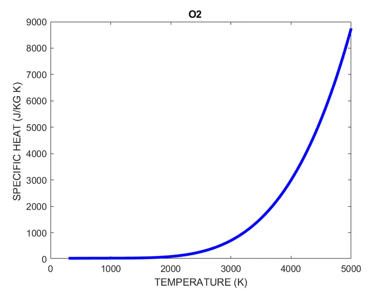
OUTPUT OF O2:

ENTHALPY:

ENTROPY:

SPECIFIC HEAT:

 

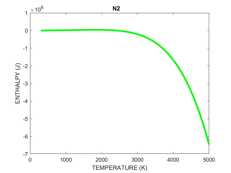
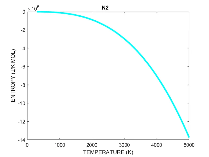
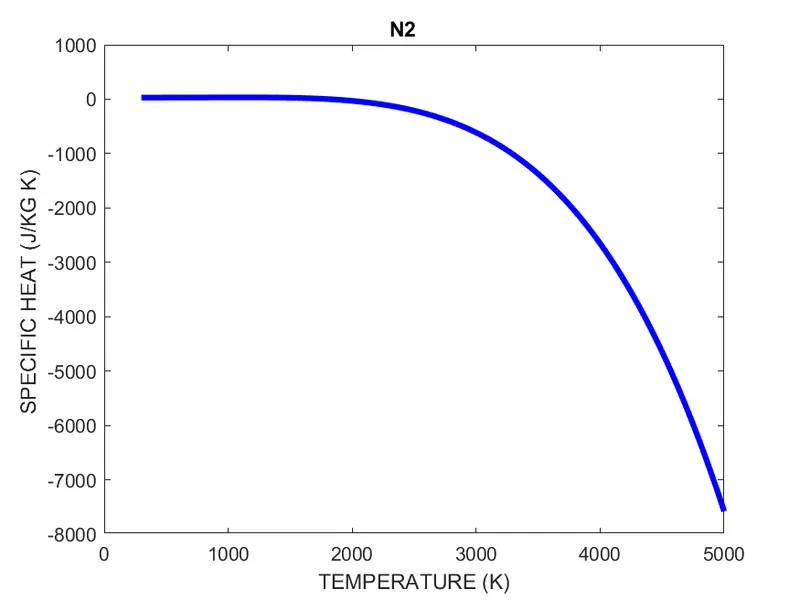
OUTPUT FOR N2:

ENTHALPY:

ENTROPY:

SPECIFIC HEAT:

 

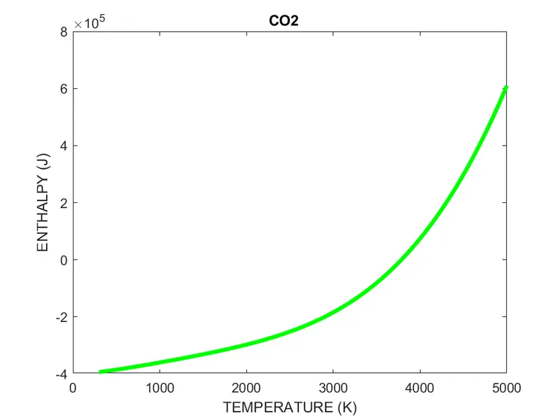
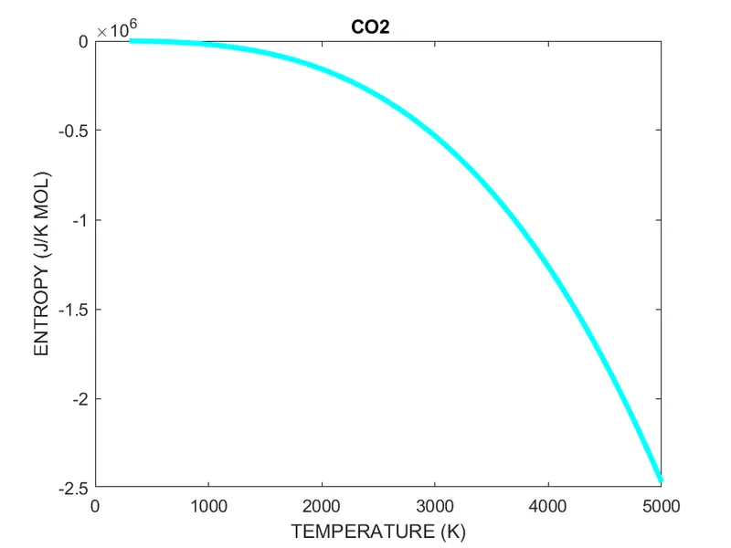
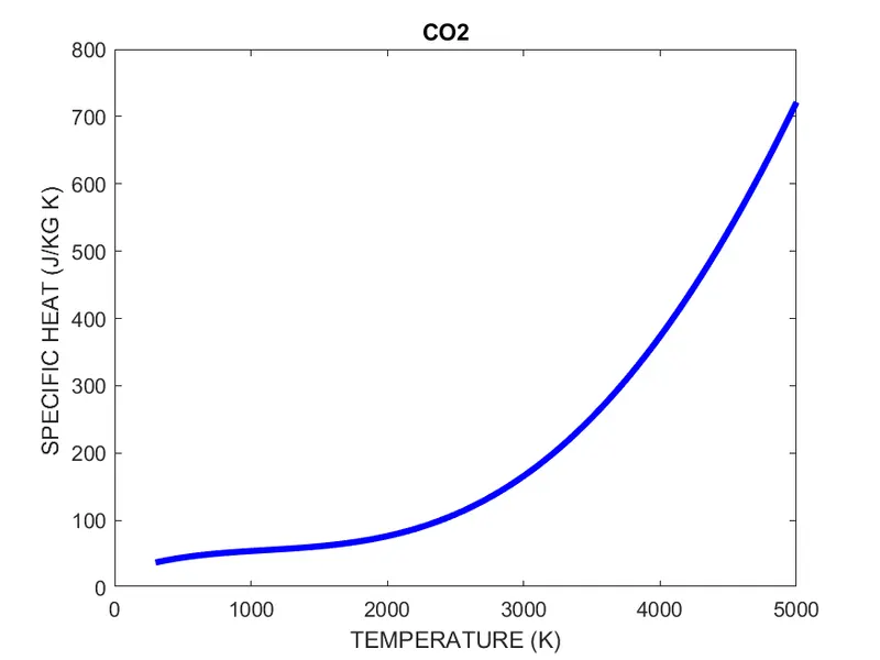
OUTPUT FOR CO2:

ENTHALPY:

ENTROPY:

SPECIFIC HEAT:

 

CONCLUSION:

               Thus the file parsing of NASA thermodynamic data has been done using MATLAB.