Week 3 - Solving second order ODEs

AIM:

To write a code for creating a animation of simple pendulum using matlab.

EXPLANATION:

SIMPLE PENDULUM:

A pendulum is a weight suspended from a pivot so that it can swing freely. When a pendulum is displaced sideways from its resting, equilibrium position, it is subject to a restoring force due to gravity that will accelerate it back toward the equilibrium position. When released, the restoring force acting on the pendulum's mass causes it to oscillate about the equilibrium position, swinging back and forth. The time for one complete cycle, a left swing and a right swing, is called the period. The period depends on the length of the pendulum and also to a slight degree on the amplitude, the width of the pendulum's swing.

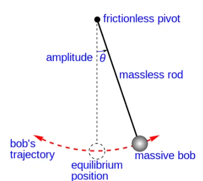
SIMPLE PENDULUM

Simple pendulum equation,

`(d^2 θ)/dt^2 +b/m (d θ)/dt+g/l sinθ=0` .......(1)

Where,

g=gravity in (m/s^2),

l=length of pendulum in (m),

m=mass of the ball in (kg),

b=damping coefficient.

To solve this ode in matlab,we convert the second order ode to first order ode.

For that let us assume,

`theta =theta1`

Then,

`(dθ)/dt= (dθ1)/dt= θ2`

Now putting the assumptions in equation (1),

`(dθ2)/dt+b/m θ2+ g/l sin⁡(θ1)=0`

`(dθ2)/dt= -[b/m θ2+ g/l sin⁡(θ1)]`

We use the above equation to solve the ode in matlab.

MATLAB CODE:

clear all
close all
clc

% inputs
%damping coefficient
b=0.05;
%gravity (m/s^2)
g=9.81;
%length of string (m)
l=1;
%mass (kg) 
m=1;


% initial conditions
theta_0=[0;3];

%time points
t_span = linspace(0,20,200);

% solve ode
[t,results]=ode45(@(t,theta) ode_func(t,theta,b,g,l,m),t_span,theta_0);

%plotting
figure(1)
plot(t,results(:,1))
hold on
plot(t, results(:,2))
xlabel('time')
ylabel('theta')

legend('angular displacement','angular velocity')
hold off

ct=1;
for i=1:length(t)
    x0=0;
    y0=0;
    
    x1=l*sin(results(i,1));
    y1=-l*cos(results(i,1));
    
    figure(2)
    plot([x0 x1],[y0 y1],'color','r')
    hold on
    plot([1 -1],[0 0],'color','b')
    
    plot(x1,y1,'.','markersize',100)
    axis([-1 1 -1 1])
    pause(0.03)
    hold off
    
    M(ct)=getframe(gcf);
    ct=ct+1;
    
end
movie(M)
videofile=VideoWriter('pendulum_ode.avi','uncompressed AVI');
open(videofile)
writeVideo(videofile,M)
close(videofile)

FUNCTION CODE TO RUN THE MAIN ODE:

function [dtheta_dt]=ode_func(t,theta,b,g,l,m)

theta1 = theta(1);
theta2 = theta(2);

dtheta1_dt = theta2;
dtheta2_dt = -(b/m)*theta2 - (g/l)*sin(theta1);
dtheta_dt=[dtheta1_dt;dtheta2_dt];
end

CODE EXPLANATION:

• The inputs parameters for the program to run are defined first.
• Time interval for the motion to display is defined as time span.
• Then,ode45 command is used to solve the differential equation.
• Ode func is linked with the main program by calling its function name.
• Then countor command is used to change the looping iteration.
• The initial and maximum position of pendulum bob is founded.
• The videofile is created to show the behaviour of the pendulum.

OUTPUT:

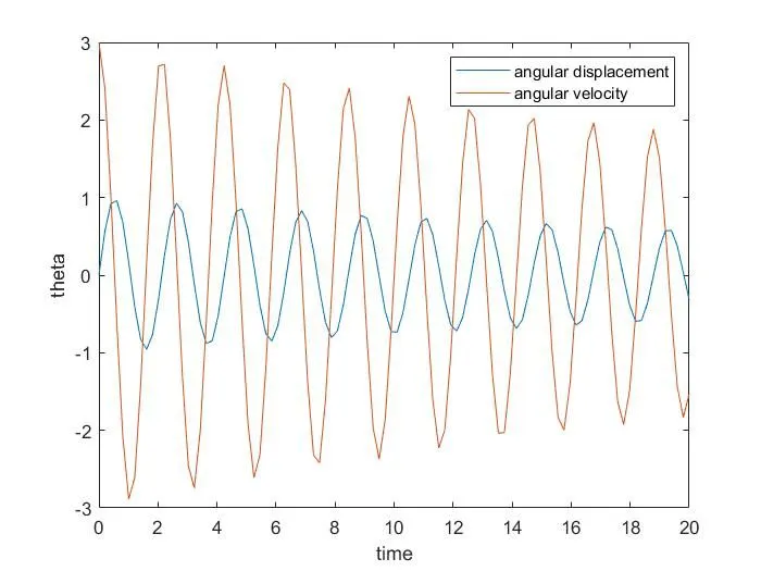
PLOT BETWEEN TIME AND THETA:

ANIMATION :

https://drive.google.com/file/d/1vjNmWmW2oNVmnl3XJ8Kc-zz0ogPxpLEA/view?usp=sharing

CONCLUSION:

Thus the transient behaviour of simple pendulum is analysed using matlab.