Simulation of a 1D Super-sonic nozzle flow simulation using McCormack Method(MATLAB)
Objective: Simulate the isentropic flow through a quasi 1D subsonic-supersonic nozzle.
Solution:
The Governing Continuity, Energy, and Momentum equations for the quasi-1D steady, isentropic flow can be expressed as;
Continuity: `rho_1 V_1A_1=rho_2V_2A_2`
Energy: `h_1+V_1/2=h_2+V_2/2`
Momentum: `P_1A_1+rho_1V_1^2A_1+int PdA=P_2A_2+rho_2V_2^2A_2`
There are different governing equations for Conservative and Non-conservative form;
For Conservation form:
Continuity: `(delp)/(delt)=-rho*(delv)/(delx) -rho*(vdel (LnA))/(delx)-(vdelp)/(delx)`
Energy: `(delv)/(delt)= -v* (delv)/(delx)-(1/gamma)*(((delT)/(delx)+(T/rho)*((delrho)/(delx)))`
Momentum: `(delT)/(delt)=-v(delT)/(delx)-(gamma-1)*T*((delv)/(delx)+v*(del LnA)/(delx))`
For Non-Conservation form:
Continuity: `del (rhoA)/ (delt)+del (rhoA)/(delx)=0`
Energy: `(del (rhoAv))/(delt)+(del(rhoAv^2+(1/gamma*rhoA)))/(delx)=1/gamma*p*(delA)/(delx)`
Momentum: `(del(rhoA(e/(gamma-1)+(gamma/2 *v^2))))/(delt)+(del(rhoAv(e/(gamma-1)+(gamma/2*v^2)+pAv)))/(delx)=0`
After getting the governing equations there are three steps to solve this problem;
- Mesh: A mesh is a barrier made up of connected strands of metal, fiber, or other flexible or ductile materials. A mesh is similar to a net or a web in that it has many attached strands. Here it is 1D problem so the x-axis is divided into n number of nodes. The 1st and last nodes are known as the values of boundary conditions and the remaining nodes are known as inner nodes.
- Discretise: For discretizing the inner nodes of the x-axis, using McCormack's explicit method.
- Solve: Finally, in the last step to solve the solution the boundary conditions for subsonic-supersonic flow and initial conditions for rho, T,v, and A are required.
Main Code:
clear all
close all
clc
%Inputs
n=31;
x=linspace(0,3,n);
throat= ((n-1)/2)+1;
nt=1400;

tic
%Function for non-conservative form
[rho,T,v,m,mach,dx,pr,rho_t,T_t,v_t,m_t,mach_t,pr_t]= non_conservative(x,n,throat);

%Simulation Time
non_conservative_simulation_time=toc

tic
%%Function for conservative form
[rho2,T2,v2,m2,mach2,pr2,dx,rho_t2,T_t2,v_t2,m_t2,mach_t2,pr_t2]= conservative(x,n,throat);

%Simulation Time
conservative_simulation_time=toc

figure(3)
plot(x,m,'r',"LineWidth",1.5)
hold on
plot(x,m2,'b',"LineWidth",1.5)
hold on
plot(x,linspace(0.579,0.579,n),'--','LineWidth',1.5)
xlabel('non-dimensional distance through nozzle(x)')
ylabel('non-dimensional mass flow rate')
s=legend('non-conservative','conservative','exact solution')
set(s,'location','northeast')
title('non-dimentional mass flow rate comparison')
grid on

xlim([0.00 3.00])
ylim([0.5780 0.5980])

figure(4)
a=subplot(4,1,1)
plot(x,mach)
hold on
plot(x,mach2,'*','color','r','markersize',3)
s=legend(a,{'non-conservative','conservative'})
set(s,'location','northeastoutside')
title('Variation of flow along x-axis')
grid on
pause(0.03)
ylabel('mach')

b=subplot(4,1,2)
plot(x,rho)
hold on
plot(x,rho2,'*','Color','r','markersize',3)
s=legend(b,{'non-conservative','conservative'})
set(s,'location','northeastoutside')
grid on
pause(0.03)
ylabel('rho')

c=subplot(4,1,3)
plot(x,T,'b','LineWidth',1)
hold on
plot(x,T2,'*','Color','r','markersize',3)
pause(0.03)
s=legend(c,{'non-conservative','conservative'})
set(s,'location','northeastoutside')
grid on
ylabel('T')

d=subplot(4,1,4)
plot(x,pr)
hold on
plot(x,pr2,'*','Color','r','markersize',3)
pause(0.03)
s=legend(d,{'non-conservative','conservative'})
set(s,'location','northeastoutside')
grid on
xlabel('non-dimensional length')
ylabel('pr')

subplot(4,1,4)
xlim([0.00 3.00])
ylim([0.00 1.00])

figure(5)
subplot(4,1,1)
plot(linspace(1,nt,nt),rho_t)
hold on
plot(linspace(1,nt,nt),rho_t2,"Color",'r')
hold on
plot(linspace(nt-400,nt+200,600),linspace(0.634,0.634,600),"Color",'k')
hold on
title('Timewise variation flow at the nozzle throat')
xlabel('no. of time steps')
ylabel('rho')
s=legend({'non-conservative','conservative','analytical solution'})
set(s,'location','northeastoutside')
grid on

subplot(4,1,2)
plot(linspace(1,nt,nt),T_t)
hold on
plot(linspace(1,nt,nt),T_t2,'Color','r')
hold on
plot(linspace(nt-400,nt+200,600),linspace(0.833,0.833,600),'Color','k')
hold on
xlabel('no. of time steps')
ylabel('T')
s=legend({'non-conservative','conservative','analytical solution'})
set(s,'location','northeastoutside')
grid on

subplot(4,1,3)
plot(linspace(1,nt,nt),pr_t)
hold on
plot(linspace(1,nt,nt),pr_t2,"Color",'r')
hold on
plot(linspace(nt-400,nt+200,600),linspace(0.528,0.528,600),'Color','k')
hold on
xlabel('no. of time steps')
ylabel('pr')
s=legend({'non-conservative','conservative','analytical solution'})
set(s,'location','northeastoutside')
grid on

subplot(4,1,4)
plot(linspace(1,nt,nt),mach_t)
hold on
plot(linspace(1,nt,nt),mach_t2,"Color",'r')
hold on
plot(linspace(nt-400,nt+200,600),linspace(1,1,600),'Color','k')
hold on
xlabel('no. of time steps')
ylabel('mach')
s=legend({'non-conservative','conservative','analytical solution'})
set(s,'location','northeastoutside')
grid on
Function for non-conservation:
function [rho,T,v,m,mach,dx,pr,rho_t,T_t,v_t,m_t,mach_t,pr_t]= non_conservative(x,n,throat)
n=31;
x = linspace(0,3,n);
dx=x(2)-x(1);
throat= ((n-1)/2)+1;

%Initial values
rho=1-0.3146*x;
T =1-0.2314*x; %T=temperature
v =(0.1+1.09*x).*T.^0.5;
a= 1+2.2*(x-1.5).^2; %a=area
gamma=1.4;

%Time Steps
nt= 1400;
dt=0.01;

%Outer time loop
for k= 1:nt

    rho_old=rho;
    v_old=v;
    T_old=T;
%Predictor methods
for i= 2:n-1
    dvdx= (v(i+1)-v(i))/dx;
    drhodx= (rho(i+1)-rho(i))/dx;
    dTdx=(T(i+1)-T(i))/dx;
    dlogadx= (log(a(i+1))-log(a(i)))/dx;
%Continuity equation
drhodt_p(i)= -rho(i)*(dvdx)-rho(i)*v(i)*dlogadx-v(i)*(drhodx);
% Momentum equation
dvdt_p(i)= -v(i)*dvdx - (1/gamma)*(dTdx + (T(i)/rho(i))*(drhodx));
%Energy equation
dTdt_p(i)= -v(i)*dTdx - (gamma-1)*T(i)*(dvdx+v(i)*(dlogadx));

%solution update
rho(i)= rho(i) + drhodt_p(i)*dt;
v(i)= v(i) + dvdt_p(i)*dt;
T(i)= T(i) + dTdt_p(i)*dt;
end
%Corrector methods
for i= 2:n-1
    dvdx= (v(i)-v(i-1))/dx;
    drhodx= (rho(i)-rho(i-1))/dx;
    dTdx=(T(i)-T(i-1))/dx;
    dlogadx= (log(a(i))-log(a(i-1)))/dx;
%Continuity equation
drhodt_c(i)= -rho(i)*(dvdx)-rho(i)*v(i)*dlogadx-v(i)*(drhodx);
% Momentum equation
dvdt_c(i)= -v(i)*dvdx - (1/gamma)*(dTdx + (T(i)/rho(i))*(drhodx));
%Energy equation
dTdt_c(i)= -v(i)*dTdx - (gamma-1)*T(i)*(dvdx+v(i)*(dlogadx));
end
%Average
drhodt= 0.5*(drhodt_p+drhodt_c);
dvdt= 0.5*(dvdt_p+dvdt_c);
dTdt= 0.5*(dTdt_p+dTdt_c);

%Final Solution update
for j= 2:n-1
    rho(j)= rho_old(j)+drhodt(j)*dt;
    v(j)= v_old(j) + dvdt(j)*dt;
    T(j)= T_old(j)+ dTdt(j)*dt;
end

%Boundary Condition
%inlet
v(1)= 2*v(2)-v(3);
%outlet
rho(n)= 2*rho(n-1)-rho(n-2);
v(n)= 2*v(n-1)-v(n-2);
T(n)= 2*T(n-1)-T(n-2);

%calculate solution
m=rho.*v.*a;
pr= rho.*T;
mach= v./((T).^0.5);

%throat values
rho_t(k)= rho(throat);
T_t(k)= T(throat);
v_t(k)= v(throat);
m_t(k)= m(throat);
mach_t(k)= mach(throat);
pr_t(k)= pr(throat);

figure(1)
if k==50
   plot(x,m,'r','LineWidth',1.5)
   hold on
elseif k==100
   plot(x,m,'b','LineWidth',1.5)
   hold on
elseif k==250
   plot(x,m,'y','LineWidth',1.5)
   hold on
elseif k==500
   plot(x,m,'k','LineWidth',1.5)
   hold on
elseif k==800
   plot(x,m,'c','LineWidth',1.5)
   hold on
elseif k==1000
   plot(x,m,'g','LineWidth',1.5)
   hold on
elseif k==1400
   plot(x,m,'m','LineWidth',1.5)
   hold on
   grid on
 title('Mass flow rate(non-conserative form) along x,at different time steps')
     xlabel('non-dimensional distance through nozzle');
     ylabel('non-dimensional mass flow rate');
     legend({'50 time steps','100 time steps','250 time steps','500 time steps','800 time steps','1000 time steps','1400 time steps'})
end
end
Function for conservation:
function [rho2,T2,v2,m2,mach2,pr2,dx,rho_t2,T_t2,v_t2,m_t2,mach_t2,pr_t2]=conservative(x,n,throat)
dx=x(2)-x(1);
%Calculate initial values
for i=1:n
    if (x(i)>=0 && x(i)<=0.5)
        rho2(i)=1;
        T2(i)=1;  %T=Temperature
    elseif (x(i)>=0.5 && x(i)<=1.5)
        rho2(i)= 1-0.366*(x(i)-0.5);
        T2(i)= 1-0.167*(x(i)-0.5);
    elseif (x(i)>=1.5 && x(i)<=3.5)
        rho2(i)= 0.634-0.3879*(x(i)-1.5);
        T2(i)= 0.833-0.3507*(x(i)-1.5);
    end
end
a=1+2.2*(x-1.5).^2; %a=area
v2= 0.59./(rho2.*a);
gamma=1.4;

% vector parameter
u1= rho2.*a;
u2 = rho2.*a.*v2;
u3= u1.*((T2./(gamma-1))+((gamma/2)*(v2.^2)));

%Time
nt=1400;

%Outer Time loop
for k=1:nt
    dt= min(0.5.*(dx./((T2.^0.5)+v2)));

    u1_old=u1;
    u2_old=u2;
    u3_old=u3;
    %Flux terms
    f1=u2;
    term= (((gamma-1)/gamma)*(u3-((gamma/2)*(u2.^2./u1))));
    f2= ((u2.^2./u1)+term);
    f3=((gamma*u2.*u3)./u1)-(gamma*(gamma-1)*(u2.^3))./(2*u1.^2);

    %predictor method
    for i= 2:n-1
        df1dx(i)= (f1(i+1)-f1(i))/dx;
        df2dx(i)= (f2(i+1)-f2(i))/dx;
        df3dx(i)= (f3(i+1)-f3(i))/dx; %dlogadx(i)= (log(a(i+1))-log(a(i)))/dx

    %Source term
    dadx(i)= (a(i+1)-a(i))/dx;
    j2(i) = (1/gamma)*(rho2(i)*T2(i))*dadx(i);

    % continuity equation
    du1dt_p(i)= -df1dx(i);
    % momentum equation
    du2dt_p(i)= -df2dx(i)+ j2(i);
    %energy equation
    du3dt_p(i)= -df3dx(i);

    %solution update
    u1(i)= u1(i)+ du1dt_p(i)*dt;
    u2(i)= u2(i)+ du2dt_p(i)*dt;
    u3(i)= u3(i)+ du3dt_p(i)*dt;
    end
 %decoding primitive terms to initialize the corrector step
 rho2= u1./a;
 v2= u2./u1;
 T2= (gamma-1)*((u3./u1)-((gamma*v2.^2)/2));

  %Flux terms
    f1=u2;
    term= (((gamma-1)/gamma)*(u3-((gamma/2)*(u2.^2./u1))));
    f2= ((u2.^2./u1)+term);
    f3=((gamma*u2.*u3)./u1)-(gamma*(gamma-1)*(u2.^3))./(2*u1.^2);

    %corector method
    for i= 2:n-1
        df1dx(i)= (f1(i)-f1(i-1))/dx;
        df2dx(i)= (f2(i)-f2(i-1))/dx;
        df3dx(i)= (f3(i)-f3(i-1))/dx; %dlogadx(i)= (log(a(i+1))-log(a(i)))/dx

    %Source term
    dadx(i)= (a(i)-a(i-1))/dx;
    j3(i) = (1/gamma)*(rho2(i)*T2(i))*dadx(i);

    % continuity equation
    du1dt_c(i)= -df1dx(i);
    % momentum equation
    du2dt_c(i)= -df2dx(i)+ j3(i);
    %energy equation
    du3dt_c(i)= -df3dx(i);
    end
    %average derivative
    du1dt= 0.5*(du1dt_p + du1dt_c);
    du2dt= 0.5*(du2dt_p + du2dt_c);
    du3dt= 0.5*(du3dt_p + du3dt_c);

    % Final solution update
    for j= 2:n-1
    u1(j)= u1_old(j)+ du1dt(j)*dt;
    u2(j)= u2_old(j)+ du2dt(j)*dt;
    u3(j)= u3_old(j)+ du3dt(j)*dt;
    end
    %Boundary Conditions
    %Inlet
    u1(1) = rho2(1)*a(1);
    u2(1) = 2*u2(2)-u2(3);
    v2(1) = u2(1)/u1(1);
    u3(1) = u1(1)*((T2(1)/(gamma-1))+((gamma/2)*v2(1)^2));
    %outlet
    u1(n) = 2*u1(n-1) - u1(n-2);
    u2(n) = 2*u2(n-1) - u2(n-2);
    u3(n) = 2*u3(n-1) - u3(n-2);

    %decoding term
    rho2 = u1./a;
    v2 = u2./u1;
    T2 = (gamma-1)*((u3./u1)-((gamma*v2.^2)/2));
    m2 = rho2.*v2.*a;
    mach2 = v2./((T2).^0.5);
    pr2 = rho2.*T2; %pressure ratio

    %throat values
    rho_t2(k) = rho2(throat);
    T_t2(k)= T2(throat);
    v_t2(k)= v2(throat);
    m_t2(k)= m2(throat);
    mach_t2(k)= mach2(throat);
    pr_t2(k)= pr2(throat);

    figure(2)
    if k==50
        plot(x,m2,'r','LineWidth',1.5)
        hold on
    elseif k==100
        plot(x,m2,'b','LineWidth',1.5)
        hold on
    elseif k==250
        plot(x,m2,'y','LineWidth',1.5)
        hold on
    elseif k==500
        plot(x,m2,'k','LineWidth',1.5)
        hold on
    elseif k==800
        plot(x,m2,'c','LineWidth',1.5)
        hold on
    elseif k==1000
        plot(x,m2,'g','LineWidth',1.5)
        hold on
    elseif k==1400
        plot(x,m2,'m','LineWidth',1.5)
        hold on
        grid on
     title('Mass flow rate(conserative form) along x,at different time steps')
     xlabel('non-dimensional distance through nozzle');
     ylabel('non-dimensional mass flow rate');
     legend({'50 time steps','100 time steps','250 time steps','500 time steps','800 time steps','1000 time steps','1400 time steps'})
    end
    end
PLOTS:
1. Variation of Mass flow rate distribution inside the nozzle at different time steps during the time-marching process.
1.1 For non-conservative form:
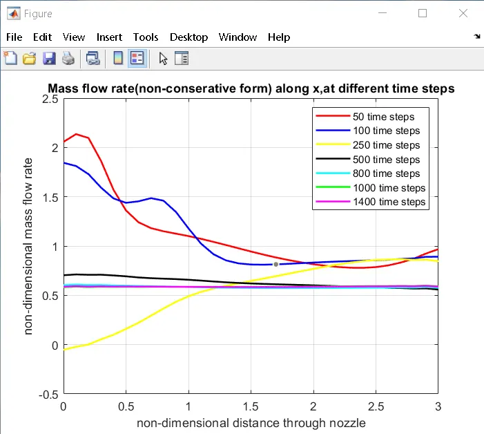
- From the above plot, it can be observed that mass flow rate curves are almost overlapping for time step 800, 1000 & 1400. It is seen that after 800-time steps, steady-state is obtained for non-conservative form.
1.2 For non-conservative form:
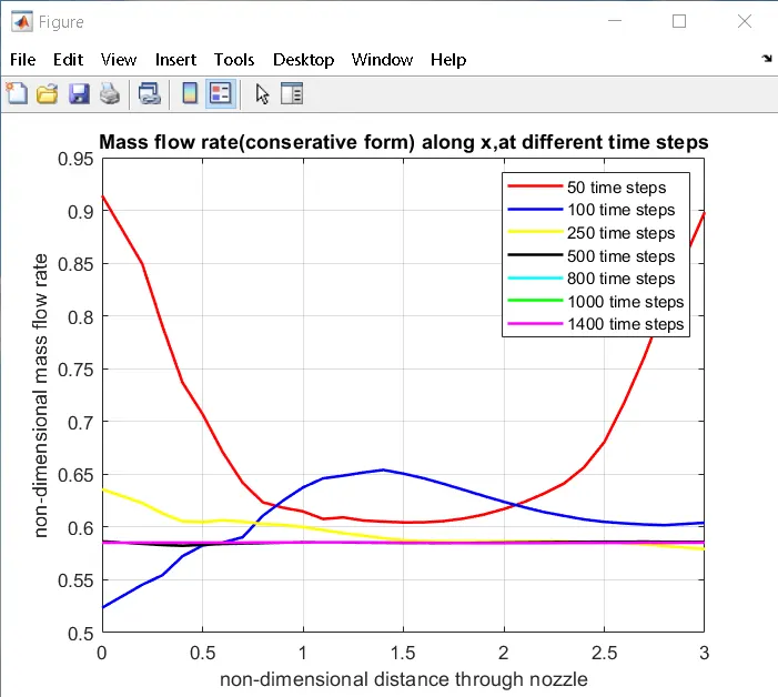
- From the above plot, it can be observed that mass flow rate curves are almost overlapping for time step 500, 800, 1000 & 1400. When compared to the non-conservative plot, the fluctuations are less compared to the conservative plot.
2. Comparison of Non-dimensional mass flow rate:
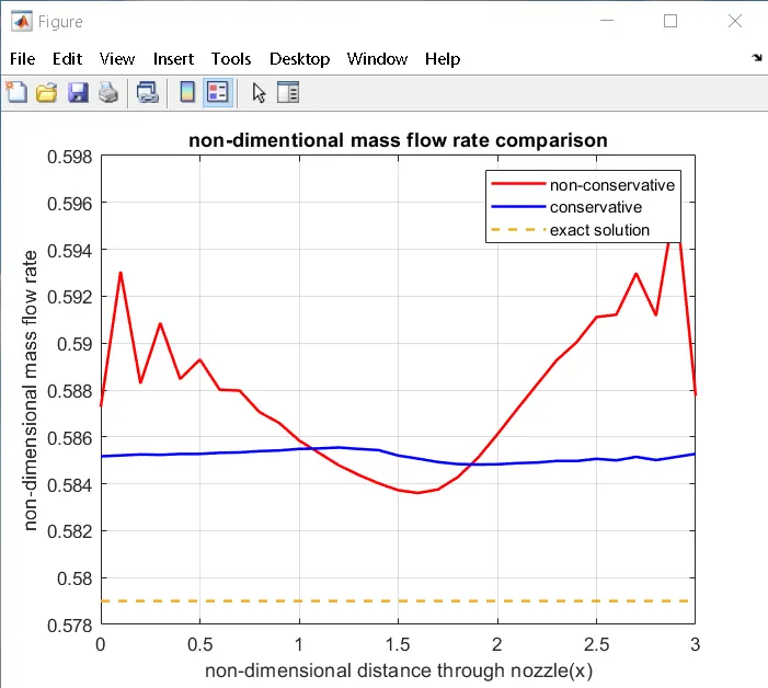
- The conservative form of the equation gives better results for mass flow rate than the non-conservative form.
3. Distribution of primitive variables inside the nozzle:
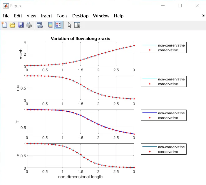
- The above plot shows the variation of flow along the x-axis with different primitive variables. It is seen that after 1400 time-steps carried out by time marching, both the forms show similar plots.
4.Time-wise variation of the primitive variables:
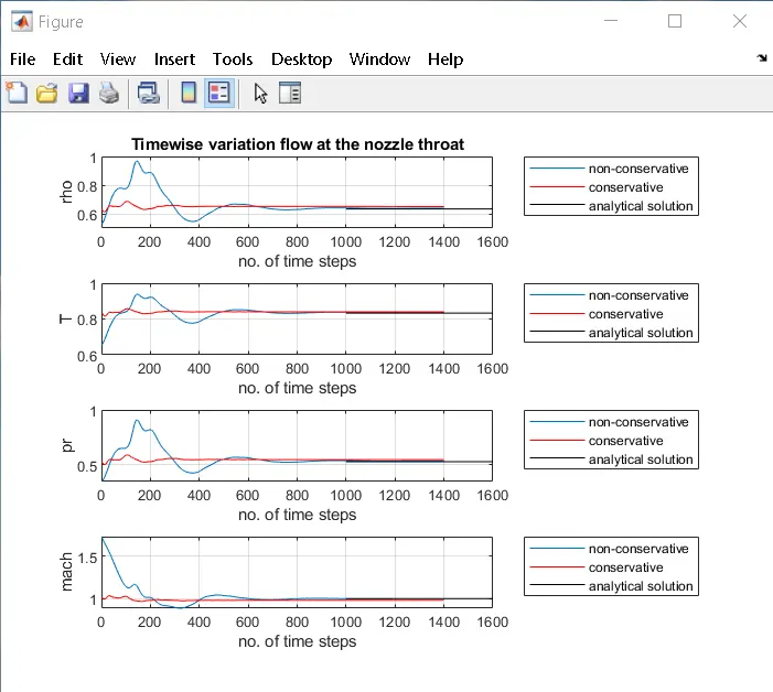
- The above plot shows, Time-wise variation of the primitive variables. From the above plot, it is seen that steady-state is obtained almost after 600-time steps.
Conclusion:
- In this project, we have successfully simulated isentropic flow through a quasi 1D subsonic-supersonic nozzle. Here, we have derived both the conservation and non-conservation forms of the governing equations and solved them using MacCormack's technique.
- Differences between the two forms of governing equations were compared with their solutions.
References:
1.Computations Fluid Dynamics: The Basics and Applications- John D. Anderson