Taylor table method and MATLAB code

Objective: Write a program in Matlab to evaluate the second-order derivative of the analytical function exp(x)*cos(x) and compare it with the 3 numerical approximations that you have derived.

Theory:

1.Skewed right-sided difference:

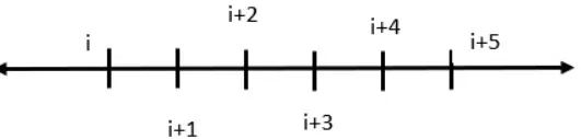
	f(i)	f'(i)*Δ(x)	f''(i)*Δ(x)^2	f'''(i)Δ(x)^3	f''''(i)Δ(x)^4	f'''''(i)Δ(x)^5
f(i)	a	0	0	0	0	0
f(i+1)	b	b	b/2	b/6	b/24	b/120
f(i+2)	c	2c	4c/2	8c/6	16c/24	32c/120
f(i+3)	d	3d	9d/2	27d/6	81d/24	243d/120
f(i+4)	e	4e	16e/2	64e/6	256e/24	1024e/120
f(i+5)	g	5g	25g/2	125g/6	625g/24	3125g/120
	0	0	1	0	0	0

2.Skewed left-sided difference:

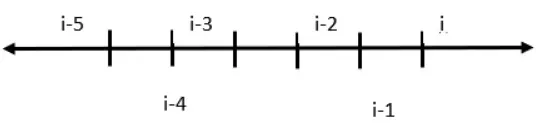
	f(i)	f'(i)*Δ(x)	f''(i)*Δ(x)^2	f'''(i)Δ(x)^3	f''''(i)Δ(x)^4	f'''''(i)Δ(x)^5
f(i)	a	0	0	0	0	0
f(i-1)	b	-b	b/2	-b/6	b/24	-b/120
f(i-2)	c	-2c	4c/2	-8c/6	16c/24	-32c/120
f(i-3)	d	-3d	9d/2	-27d/6	81d/24	-243d/120
f(i-4)	e	-4e	16e/2	-64e/6	256e/24	-1024e/120
f(i-5)	f	-5g	25g/2	-125g/6	625g/24	-3125g/120
	0	0	1	0	0	0

3. Central difference

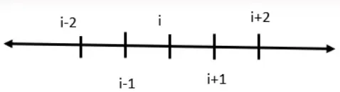
	f(i)	f'(i)*Δ(x)	f''(i)*Δ(x)^2	f'''(i)Δ(x)^3	f''''(i)Δ(x)^4
f(i-2)	a	-2a	4a/2	-8a/6	0
f(i-1)	b	-b	b/2	-b/6	b/24
f(i)	c	0	0	0	0
f(i+1)	d	d	d/2	d/6	d/24
f(i+2)	e	2e	4e/2	8e/6	16e/24
		0	1	0	0

CODE:

clear all
close all
clc
% Initial Parameter
x= pi/3;
dx=linspace(pi/4,pi/400,100);
%Analytical Function = exp^(x)*cos(x)
analytical_derivative= -2*exp(x)*sin(x);

for i=1:length(dx)
    %Taylor series function at various node points
    a(i)=(exp(x-(5*dx(i)))*cos(x-(5*dx(i))));
    b(i)=(exp(x-(4*dx(i)))*cos(x-(4*dx(i))));
    c(i)=(exp(x-(3*dx(i)))*cos(x-(3*dx(i))));
    d(i)=(exp(x-(2*dx(i)))*cos(x-(2*dx(i))));
    e(i)=(exp(x-dx(i))*cos(x-dx(i)));
    f(i)=(exp(x)*cos(x));
    g(i)=(exp(x+dx(i))*cos(x+dx(i)));
    h(i)=(exp(x+(2*dx(i)))*cos(x+(2*dx(i))));
    j(i)=(exp(x+(3*dx(i)))*cos(x+(3*dx(i))));
    k(i)=(exp(x+(4*dx(i)))*cos(x+(4*dx(i))));
    l(i)=(exp(x+(5*dx(i)))*cos(x+(5*dx(i))));
    
    %Expression Formula
    %Central difference 
    CDS(i)=(-1*(d(i))+16*(e(i))-30*(f(i))+16*(g(i))-1*(h(i)))/(12*(dx(i)^2));
    
    %Skewed Left Side difference
    skew_left(i)=(45*(f(i))-154*(e(i))+214*(d(i))-156*(c(i))+61*(b(i))-10*(a(i)))/(12*(dx(i)^2));
    
    %Skewed Right Side difference
    skew_right(i)=(45*(f(i))-154*(g(i))+214*(h(i))-156*(j(i))+61*(k(i))-10*(l(i)))/(12*(dx(i)^2));
    
    error_CDS(i)=abs(CDS(i)-analytical_derivative);
    error_LDS(i)=abs(skew_left(i)-analytical_derivative);
    error_RSD(i)=abs(skew_right(i)-analytical_derivative);
     
end

%Plotting
loglog(dx,error_CDS,'linewidth',1,'marker','diamond');
hold on
loglog(dx,error_LDS,'linewidth',1,'marker','hexagram');

loglog(dx,error_RSD,'linewidth',1,'marker','pentagram');
xlabel('Value of dx')
ylabel('Absolute error')
legend('Central Difference','Skewed left side difference','skewed right side difference')

OUTPUT:

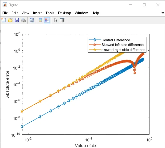
why a skewed scheme is useful? What can a skewed scheme do that a CD scheme cannot?

As we can see from the figure central difference gives the least error but this scheme cannot be used in boundary regions where there won't be succeeding or preceding points. Hence for such conditions skewed scheme is useful depending on the points situated either left or right.

Conclusion:

Thus fourth-order approximations are derived for a second-order derivative using the Taylors table method by providing suitable MATLAB code.