Rankine cycle Simulator(MATLAB)

Objective:

1. Creating a Rankine cycle simulator & calculating the state points based on user input's.
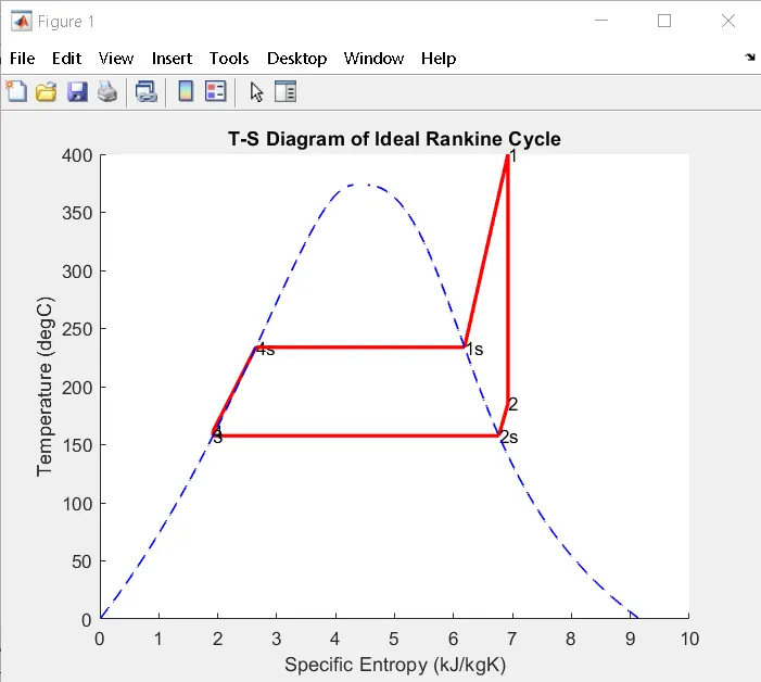
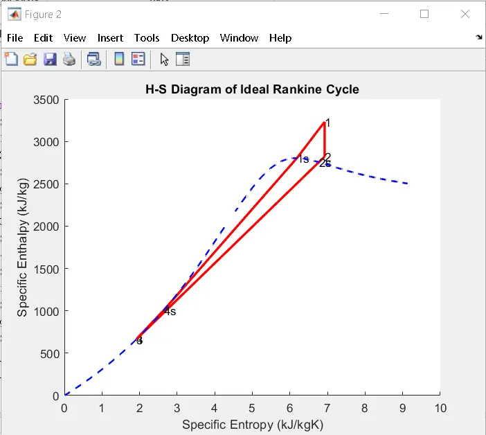
2. Plotting the corresponding T-S and H-S plot.

Theory:

Rankine cycle is the theoretical cycle on which steam turbine works.Rankine cycle is the process widely used by power plants such as coal fired power plants or nuclear reactor. In this mechanism, a fuel is used to produce heat within a boiler, converting water into steam which then expands through a turbine producing useful work. This process was developed in 1859 by Scottish engineer William J.M. Rankine.

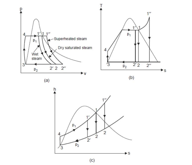
Following process takes place in rankine cycle ;

Process 1-2: Reversible adiabatic expansion in the turbine.

Process 2-3: Constant-Pressure transfer of heat in the condenser.

Process 3-4: Reversible adiabatic pumping process in the feed pump.

Process 4-1: Constant-Pressure transfer of heat in the boiler.

Applying Steady flow energy equation (S.F.E.E),neglecting K.E & P.E;

1. For Boiler,we get;

hf4+Q1=h1

∴Q1=h1-hf4

2.For Turbine,we get;

h1 =WT+h2 where WT=Turbine work

∴WT=h1-h2

3. For Condenser,we get;

h2=Q2+hf3

∴Q2=h2-hf3

4. For feed pump,we get;

hf3+Wp=hf4 where Wp=Pump work

∴Wp=hf4-hf3

Efficiency of Rankine Cycle is given by;

η=Wnet/Qin *100

Specific Steam Consumption is given by;

SSC=3600/WT

Program Code:

clear all 
close all 
clc

%Process discription
fprintf('RANKINE CYCLE SIMULATORn')
fprintf('1-2 Isentropic Expansion in the Turbinen')
fprintf('2-3 Constant Pressure Heat Rejection by the Condensern')
fprintf('3-4 Isentropic Compression in the pumpn')
fprintf('4-1 Constant Pressure Heat addition by the Boilern')

%Taking all inputs
P1= input('Enter the Pressure at the Turbine inlet(in bar):');
T1= input('Enter the Temperature at the Turbine inlet(in degree celsius):');
P2= input('Enter the Pressure at the Condenser inlet(in bar):');
fprintf('Resultn')

%Calculation
%Calculation of Cp value at P1&P2 for saturated liquid&vapour
CP1_L=XSteam('CpL_p',P1);
CP1_V=XSteam('CpV_p',P1);
CP2_L=XSteam('CpL_p',P2);
CP2_V=XSteam('CpV_p',P2);

%Calculation of Saturation Temperature at P1 & P2
Tsat_P1=XSteam('Tsat_p',P1);
Tsat_P2=XSteam('Tsat_p',P2);

%Calculation of Enthalpy and Entropy at saturation points

%Calculation of saturation properties at state 1
Hg_1=XSteam('hV_p',P1);
Sg_1=XSteam('sV_p',P1);

%Calculation of saturation properties at state 2
Hg_2=XSteam('hV_p',P2);
Sg_2=XSteam('sV_p',P2);

%Calculation of saturation properties at state 3
Hf_3=XSteam('hL_p',P2);
Sf_3=XSteam('sL_p',P2);

%Calculation of saturation properties at state 4
Hf_4=XSteam('hL_p',P1);
Sf_4=XSteam('sL_p',P1);

%Calculation of process properties at state 1
fprintf('At State point 1n');
fprintf('P1 is :%f Barn',P1);
fprintf('T1 is :%f degCn',T1);

H1=XSteam('h_pT',P1,T1);
fprintf('H1 is :%f kJ/kg n',H1);

S1=XSteam('s_pT',P1,T1);
fprintf('S1 is :%f kJ/kg n',S1);

%Calculation of process properties at state 2
fprintf('At State point 2n');
fprintf('P2 is :%f Barn',P2);

S2=S1;
fprintf('S2 is :%f kJ/kg n',S2)

%Calculating the value of X
if (S2<=Sg_2)
    X2= (S2-Sf_3)/ (Sg_2-Sf_3);   %Dryness fraction at state 2
else
    X2=1;
end 
fprintf('X2 is :%f n',X2)

%Calculating the value of T2
if (X2<1)
    T2=Tsat_P2;
else
    %S2=Sg_2+CP2_V*(log(T2/Tsat_P2))
    T2=(Tsat_P2+273.15)* exp((S2-Sg_2)/CP2_V);
    T2=T2-273.15;
end
fprintf('T2 is :%f degCn',T2)

if (X2<1)
    H2= Hf_3 + X2 *(Hf_3-Hg_2);
else
    H2=XSteam('h_pT',P2,T2);
end
fprintf('H2 is :%f kJ/kg n',H2)

%Calculation of process properties at state 3
fprintf('At State point 3n')

P3=P2;
fprintf('P3 is :%f Barn',P3)

V3= XSteam('vL_p',P3);
T3=Tsat_P2;    %No subcooling assumed
fprintf('T3 is :%f degCn',T3)

H3=Hf_3;
fprintf('H3 is :%f kJ/kg n',H3)

S3=Sf_3;
fprintf('S3 is :%f kJ/kg n',S3)

%Calculation of process properties at state 4
fprintf('At State point 4n')

P4=P1;
fprintf('P4 is :%f Barn',P4)

S4=S3;
fprintf('S4 is :%f kJ/kg n',S4)

Wp= V3 * (P4-P3)*100;
H4= Wp+H3;
fprintf('H4 is :%f kJ/kg n',H4)

T4=(Tsat_P1+273.15)/(exp((Sf_4-S4)/CP1_L));
T4=T4-273.15;
fprintf('T4 is :%f degCn',T4)

%Calculation for plotting saturation liquid and vapour lines

temp= linspace(1,T1,1000);
for i=1:length(temp)
    H_L(i)= XSteam('hL_T', temp(i));
    H_V(i)= XSteam('hV_T', temp(i));
    S_L(i)= XSteam('sL_T', temp(i));
    S_V(i)= XSteam('sV_T', temp(i));
end

%Ploting T-S and H-s Diagram
%Plotting T-S Diagram

figure(1)
hold on
plot([S1 S2], [T1 T2],'r','linewidth',2)
text(S1,T1,'1')
text(S2,T2,'2')
plot([S2 Sg_2], [T2 Tsat_P2],'r','linewidth',2)
text(Sg_2, Tsat_P2,'2s')
plot([Sg_2 S3],[Tsat_P2 T3], 'r','linewidth',2)
text(S3,T3,'3')
plot([S3 S4],[T3 T4],'r','linewidth',2)
text(S4,T4,'4')
plot([S4,Sf_4],[T4 Tsat_P1],'r','linewidth',2)
text(Sf_4,Tsat_P1,'4s')
plot([Sf_4 Sg_1],[Tsat_P1 Tsat_P1],'r','linewidth',2)
text(Sg_1,Tsat_P1,'1s')
plot([Sg_1 S1],[Tsat_P1 T1],'r','linewidth',2)
plot(S_L,temp,'b','linestyle','--','linewidth',1)
plot(S_V,temp,'b','linestyle','--','linewidth',1)

title('T-S Diagram of Ideal Rankine Cycle')
ylabel('Temperature (degC)')
xlabel('Specific Entropy (kJ/kgK)')

%Plotting H-S Diagram

figure(2)
hold on 
plot([S1 S2], [H1 H2],'r','linewidth',2)
text(S1,H1,'1')
text(S2,H2,'2')
plot([S2 Sg_2], [H2 Hg_2],'r','linewidth',2)
text(Sg_2, Hg_2,'2s')
plot([Sg_2 S3],[Hg_2 H3], 'r','linewidth',2)
text(S3,H3,'3')
plot([S3 S4],[H3 H4],'r','linewidth',2)
text(S4,H4,'4')
plot([S4,Sf_4],[H4 Hf_4],'r','linewidth',2)
text(Sf_4,Hf_4,'4s')
plot([Sf_4 Sg_1],[Hf_4 Hg_1],'r','linewidth',2)
text(Sg_1,Hg_1,'1s')
plot([Sg_1 S1],[Hg_1 H1],'r','linewidth',2)
plot(S_L,H_L,'b','linestyle','--','linewidth',1.5)
plot(S_V,H_V,'b','linestyle','--','linewidth',1.5)

title('H-S Diagram of Ideal Rankine Cycle')
ylabel('Specific Enthalpy (kJ/kg)')
xlabel('Specific Entropy (kJ/kgK)')

%Calculation of Workdone,Specific Steam Consumption(SSC) and Efficiency
Wt= H1-H2;
fprintf('Work by turbine is:%f kJ/kgn',Wt)
fprintf('Work by compressor is:%f kJ/kgn',Wp)
Wnet= Wt-Wp;
fprintf('Net Workdone is:%f kJ/kgn',Wnet)
Qin= H1-H4;
efficiency_thermal= Wnet*100/Qin ;
fprintf('Thermal efficiency is:%f',efficiency_thermal);
disp('%')
SSC= 3600/Wt;
fprintf('SSC is:%f kg/kwh',SSC)

Code Explanation:

For this prgram,using XSream.m file which is basically steam table.

1. Starting with clear all,close all & clc and then by using fprintf command for printing description of all process in command window.
2. Taking all inputs.
3. Calculation of cpvalue at P1&P2 for saturation liquid and vapour.
4. Calculating Saturation temperature at P1&P2.
5. Calculations of saturation properties at state 1,2,3&4.
6. Calculations of process properties at state 1,2,3&4.
7. Calculating & plotting saturation liquid and vapour lines.
8. Plotting T-S & H-S diagram.
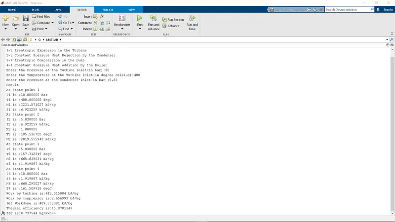
9. Calculation of workdone,efficiency and Specific Steam Consumption.

Results:

1. Plot

2. Command window: