Week 7 - Simulation of a 1D Super-sonic nozzle flow simulation using Macormack Method

Aim: To simulate the isentropic flow through a quasi 1D subsonic-supersonic nozzle.To determine the steady-state temperature distribution for the flow-field variables and investigate the difference between the two forms of governing equations i.e Non-conservative and Conservative form by comparing their solutions.

The following plots should be presented

1. Steady-state distribution of primitive variables inside the nozzle.
2. Time-wise variation of the primitive variables.
3. Variation of Mass flow rate distribution inside the nozzle at different time steps during the time-marching process.
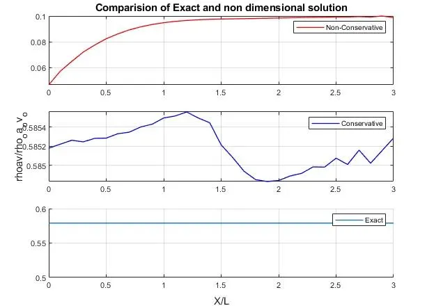
4. Comparison of Normalized mass flow rate distributions of both forms.

Introduction:

• 1D Super-sonic nozzle flow is not actually present in the real world it is just assumed to simulate the flow through nozzle.1D flow is aflow in wich the properies vary only in one direction or we consider flow in only one direction.
• The nozzle we consider is convergent divergent nozzle.
• Derivation of the conservative and Non-Conservative forms are derived.
• considering a small part in the nozzle dx an performing integration gives us the required equations.

Final non-Dimensional equations for non conservative part:

Continuity equation:

`(partialrho')/(partialt')= -rho'(partialv')/(partialx')-rho'v'partial(lnA')/(partialx')-v'(partialrho')/(partialx')`

Momentum equation:

`(partialv')/(partialt')=-v'(partialv')/(partialx')-1/gamma((partialT')/(partialx')+(T')/(rho').(partialrho')/(partialx'))`

Energy equation:

`(partialT')/(partialv')=-v'.(partialT')/(partialx')-(gamma-1)T'.((partialv')/(partialx')+v'.(partial(ln(A')))/(partialx'))`

Final non-Dimensional equations for conservative part:

Continuity equation:

`(partial(rho'A'))/(partialt')+(partial(rho'A'v'))/(partialx')`

Momentum equation:

`(partial(rho'A'v'))/(partialt')+(partial(rho'A'v'^2+(1/gamma)p'A'))/(partialt')=1/gammap'(partialA')/(partialx')`

Matlab codes for non conservative form and conservative forms are written in two different functions

Explaination for Main code:

In this code required inputs for both the sub functions are initiated and non conservative and conservative functions are called.tic and toc commands are used to know the time for compilation of both the codes .

Main Code:

%Main Program
close all
clear all
clc

%Initialization
n = 31;
x = linspace(0,3,n);
dx = x(2)-x(1);
gamma =1.4;
%Area
a = 1+2.2*(x-1.5).^2;
%finding throat position
nthroat =find((a-1)<0.001);
CFL = 0.5;
%%%Non Conservative form
[v,t,p,rho,M,m,pthroat,vthroat,tthroat,rhothroat,k,Mthroat,mthroat,timen]=non_conservative_part(n,x,dx,a,gamma,nthroat);
Non_Conservative_simulation_time =timen

%%%Conservative form
[vs,ts,ps,rhos,Ms,ms,pthroats,vthroats,tthroats,rhothroats,k,Mthroats,mthroats,timec]=conservative_part(n,x,dx,a,gamma,CFL,nthroat);
Conservative_simulation_time = timec
%plot
fig =figure(7);
subplot(3,1,1);
title('Comparision of Exact and non dimensional solution');
plot(x,m,'r','linewidth',1);
legend('Non-Conservative');
 hold on
 grid on
 subplot(3,1,2);
plot(x,ms,'b','Linewidth',1);
legend('Conservative');
hold on
grid on
subplot(3,1,3)
line([0 3],[0.579 0.579],'linewidth',1);
grid on
axis([0 3 0.5 0.6])
legend('Exact');
han=axes(fig,'visible','off'); 
han.Title.Visible='on';
han.XLabel.Visible='on';
han.YLabel.Visible='on';
ylabel(han,'rhoav/rho_oa_ov_o');
xlabel(han,'X/L');
title(han,'Comparision of Exact and non dimensional solution');

The number of time steps is taken as 750 because there is no significant change in the plots after 700

Explaination for the non conservative form code:

1. Code begins with Function give all the variables that need to be called in the man function.
2. Initialization the values for the variables.
3. For loop is started to run the code for required timesteps.A copy of the values are kept.
4. Another for loop to run the iterations n number of times.In this loop the continuity ,momentum and energy equations are written with proper initialization.final values are added with the initial values.
5. In this step forward differencing is used.This step is called the predicter step.
6. For loop is opened for the correcter method ,in this method.similar to predicter step all the equations are iterated only difference is initial value is not added to the final and backward differencing is used.and the loop is ended.
7. In the next step average taken between the predicted step values and corrected step values
8. In the next step the average values are added with the old values which are kept as a copy.
9. Boundary conditions are applied with the help of anderson textbook data.
10. throat position is found as it is the place where Un steady state occurs.
11. Required plots are plotted.

Code for Non Conservative form:

function [v,t,p,rho,M,m,pthroat,vthroat,tthroat,rhothroat,k,Mthroat,mthroat,timen]=non_conservative_part(n,x,dx,a,gamma,nthroat)

rho = 1-0.314*x;
t = 1-0.2314*x;%t =temperature
v = (0.1+1.09*x).*t.^0.5;
a = 1+2.2*(x-1.5).^2;
%Time steps
nt =750;
dt =0.01;

tic
%outer time loop
for k =1:nt
    %predictor method
    %copy
    rho_old = rho;
    v_old = v;
    t_old = t;
    for j = 2:n-1 ;
        dvdx = (v(j+1)-v(j))/dx;
        drhodx = (rho(j+1)-rho(j))/dx;
        dlogadx = (log(a(j+1))-log(a(j)))/dx;
        dtdx = (t(j+1)-t(j))/dx;
        %continuity Equation
        drhodt_p(j) = -rho(j)*dvdx-rho(j)*v(j)*dlogadx-v(j)*drhodx;
        %Momentum Equation
        dvdt_p(j) = -v(j)*dvdx-(1/gamma)*(dtdx+(t(j)/rho(j))*drhodx);
        %Energy Equation
        dtdt_p(j) = -v(j)*dtdx-(gamma -1)*t(j)*(dvdx+v(j)*dlogadx);
        %solution update
        v(j) = v(j)+dvdt_p(j)*dt;
        rho(j) = rho(j)+drhodt_p(j)*dt;
        t(j) = t(j) +dtdt_p(j)*dt;
    end
        %corrector method
        for j = 2:n-1 ;
        dvdx = (v(j)-v(j-1))/dx;
        drhodx = (rho(j)-rho(j-1))/dx;
        dlogadx = (log(a(j))-log(a(j-1)))/dx;
        dtdx = (t(j)-t(j-1))/dx;
        %continuity Equation
        drhodt_c(j) = -rho(j)*dvdx-rho(j)*v(j)*dlogadx-v(j)*drhodx;
        %Momentum Equation
        dvdt_c(j) = -v(j)*dvdx-(1/gamma)*(dtdx+(t(j)/rho(j))*drhodx);
        %Energy Equation
        dtdt_c(j) = -v(j)*dtdx-(gamma -1)*t(j)*(dvdx+v(j)*dlogadx);
        end
    %compute the average time value
    dvdt = 0.5*(dvdt_p+dvdt_c);
    drhodt = 0.5*(drhodt_p+drhodt_c);
    dtdt = 0.5*(dtdt_p+dtdt_c);
    %Final solution update
    for i =2:n-1;
        v(i) = v_old(i) + dvdt(i)*dt;
        rho(i) = rho_old(i) + drhodt(i)*dt;
        t(i) = t_old(i) + dtdt(i)*dt;
    end

 %Apply boundary conditions
    %inlet
    v(1) = 2*v(2)-v(3);
    rho(1) = 2*rho(2)-rho(3);
    t(1) = 2*t(2)-t(3);
    %outlet
    v(n) = 2*v(n-1)-v(n-2);
    rho(n) = 2*rho(n-1)-rho(n-2);
    t(n) = 2*t(n-1)-t(n-2);
   
    %Defining mass flow rate,presuure,mach number
    p = rho.*t; %pressure
    m = rho.*a.*v; %Mass flow rate
    M = v./sqrt(t); %mach number
    
    %parameters at throat
    tthroat(k) = t(nthroat);
    pthroat(k) = p(nthroat);
    rhothroat(k) = rho(nthroat);
    mthroat(k) = m(nthroat);
    vthroat(k) = v(nthroat);
    Mthroat(k) = M(nthroat);
    %comparing mass flow rates at various time steps
    figure(1);
    hold on
    if k==50
        plot(x,m,'b');
    elseif k==100
        plot(x,m,'m');
    elseif k==150
        plot(x,m,'g');
    elseif k==200
        plot(x,m,'r');
    elseif k==700
        plot(x,m,'c');
        end
end
 timen = toc; 
legend('t=50','t=100','t=150','t=200','t=700','location','best');
xlabel('x/L');
ylabel('Mass flow rate(rhoav/rho_oa_ov_o)');
title('variation in mass flow rate W.R.T time');

%Primitive properties at unsteady state (Throat section)
figure(2);
%Density
subplot(4,1,1)
plot(rhothroat,'b');
legend('Density');
title('Properties at un Steady-State (Throat section)')
ylabel('rho/rho_o');
axis([0 750 0 0.9]);
%Pressure
subplot(4,1,2)
plot(pthroat,'m');
legend('Pressure');
ylabel('P/P_o');
axis([0 750 0 0.9]);
%Temperature
subplot(4,1,3)
plot(tthroat,'c');
legend('Temperature');
ylabel('T/T_o');
axis([0 750 -0.1 1]);
%Mach number
subplot(4,1,4)
plot(Mthroat,'k');
legend('Mach number');
ylabel('M/M_o');
axis([0 750 -0.1 1.6]);

%Steady state properties
figure(3);
%Density
subplot(4,1,1)
plot(x,rho,'b');
legend('Density');
title('Steady state properties')
ylabel('rho/rho_o');
axis([0 3 -0.1 0.3]);
%Pressure
subplot(4,1,2)
plot(x,p,'m');
legend('Pressure');
ylabel('P/P_o');
axis([0 3 -0.1 0.2]);
%Temperature
subplot(4,1,3)
plot(x,t,'c');
legend('Temperature');
ylabel('T/T_o');
axis([0 3 0 0.7]);
%Mach number
subplot(4,1,4)
plot(x,M,'k');
legend('Mach number','location','best');
ylabel('M/M_o');
axis([0 3 -0.1 5]);
xlabel('Length(X/L)')

Explaination for the conservative form code:

1. Code begins with Function give all the variables that need to be called in the man function.
2. Initialization the values for the variables. different x values are given using if else looping.A copy of the values are kept.
3. Definitions of U1,U2,U3 are given.
4. For loop is started to run the code for required timesteps.U1,U2,u3 values are kept acopy.F1,F2,F3 are defined
5. Another for loop (Predicter step)to run the iterations n number of times.In this loop the continuity ,momentum and energy equations are written with proper initialization.Updation of U1,U2,U3 are done.
6. In this step forward differencing is used.This step is called the predicter step.
7. For loop is opened for the correcter method ,in this method.similar to predicter step all the equations are iterated only difference is initial value is not added to the final.and the loop is ended.And also Backward differencing is used.
8. In the next step average taken between the predicted step values and corrected step values
9. In the next step the average values are added with the old values which are kept as a copy.
10. Boundary conditions are applied with the help of anderson textbook data.
11. throat position is found as it is the place where Un steady state occurs.
12. Required plots are plotted.

Matlab Code for Consrvative form:

%Solving 1D supersonic and subsonic Nozzle flow in conservative form

function [vs,ts,ps,rhos,Ms,ms,pthroats,vthroats,tthroats,rhothroats,k,Mthroats,mthroats,timec]=conservative_part(n,x,dx,a,gamma,CFL,nthroat);
%initialization
nt = 1400;
dt =0.001;
tic
for i = 1:length(x)
    if x(i)>=0&&x(i)<0.5
        rhos(i) = 1;
        ts(i) = 1;
    elseif x(i)>=0.5&&x(i)<1.5
        rhos(i) = 1-0.366*(x(i)-0.5);
        ts(i) = 1-0.167*(x(i)-0.5);
    elseif x(i)>=1.5&&x(i)<=3
        rhos(i) = 0.634-0.3879*(x(i)-1.5);
        ts(i) = 0.833-0.3507*(x(i)-1.5);
    end
end

rho = rhos;
t = ts;
vs = (0.59)./(rhos.*a);
u = vs;

rho_olds = rhos;
t_olds = ts;
v_olds = vs; 

%initial conditions
u1 = rhos.*a;
u2 = rhos.*a.*vs;
u3 = rhos.*a.*((ts./(gamma-1))+((gamma/2)*(vs.^2)));

%Time looping
for k = 1:nt
    u1old  = u1;
    u2old = u2;
    u3old = u3;
    
    dts = CFL*(dx./(sqrt(ts)+vs));
    dt = min(dts);
    
    f1 = u2;
    f2 = ((u2.^2)./u1)+(((gamma-1)/gamma)*(u3-((gamma*0.5*(u2.^2))./u1)));
    f3 = ((gamma*u2.*u3)./u1)-((gamma*0.5*(gamma-1)*(u2.^3))./(u1.^2));
    %predector step
    for j = 2:n-1
        J2(j) = (1/gamma)*rhos(j)*ts(j)*((a(j+1)-a(j))/dx);
        
        %continuity Equation
        du1dts_p(j) = -(f1(j+1)-f1(j))/dx;
        %Momentum Equation
        du2dts_p(j) = -((f2(j+1)-f2(j))/dx)+J2(j);
        %Energy Equation
        du3dts_p(j) = -(f3(j+1)-f3(j))/dx;
        
        %updating solution
        u1(j) = u1(j)+du1dts_p(j)*dt;
        u2(j) = u2(j)+du2dts_p(j)*dt; 
        u3(j) = u3(j)+du3dts_p(j)*dt;
    end
    
        %Predicted values
        rhos = u1./a;
        vs = u2./u1;
        ts = (gamma-1)*((u3./u1)-((gamma/2)*((u2./u1).^2)));
        ps = rhos.*ts;
        
        f1 = u2;
        f2 = ((u2.^2)./u1)+(((gamma-1)/gamma)*(u3-((gamma*0.5*(u2.^2))./u1)));
        f3 = ((gamma*u2.*u3)./u1)-((gamma*0.5*(gamma-1)*(u2.^3))./(u1.^2));
        
        %corrector step
        for j = 2:n-1
        J2(j) = (1/gamma)*rhos(j)*ts(j)*((a(j)-a(j-1))/dx);
        
        %continuity Equation
        du1dts_c(j) = -(f1(j)-f1(j-1))/dx;
        %Momentum Equation
        du2dts_c(j) = -((f2(j)-f2(j-1))/dx)+J2(j);
        %Energy Equation
        du3dts_c(j) = -(f3(j)-f3(j-1))/dx;
        end
        
        %Computing Avarage time derivative
        du1dts = 0.5*(du1dts_p + du1dts_c);
        du2dts = 0.5*(du2dts_p + du2dts_c);
        du3dts = 0.5*(du3dts_p + du3dts_c);
        
        %Final solution update
        for i = 2:n-1
            u1(i) = u1old(i)+du1dts(i)*dt;
            u2(i) = u2old(i)+du2dts(i)*dt;
            u3(i) = u3old(i)+du3dts(i)*dt;
        end
        
        %Boundary conditions
        %In Inlet
        rhos = u1./a;
        vs = u2./u1;
        ts = (gamma-1)*((u3./u1)-((gamma/2)*((u2./u1).^2)));
        
        u1(1) = rhos(1)*a(1);
        u2(1) = 2*u2(2)-u2(3);
        u3(1) = u1(1)*(ts(1)/(gamma-1)+(gamma/2)*(vs(1)^2));
        %At Outlet
        u1(n) =2*u1(n-1)-u1(n-2);
        u2(n) =2*u2(n-1)-u2(n-2);
        u3(n) =2*u3(n-1)-u3(n-2);
        
        %Defining mass flow rate,presuure,mach number
        ps = rhos.*ts; %pressure
        Ms = vs./sqrt(ts); %Mach number
        ms = rhos.*a.*vs; %Mass flow rate
        %properties at throat
        rhothroats(k) = rhos(nthroat);
        tthroats(k) = ts(nthroat);
        Mthroats(k) = Ms(nthroat);
        vthroats(k) = vs(nthroat);
        pthroats(k) = ps(nthroat);
        mthroats(k)  = ms(nthroat); 
    %Plot showing variation in mass flow rate 
    figure(4)
    hold on
    if k==1
        plot(x,ms,'p')
    elseif k==50
        plot(x,ms,'b');
    elseif k==100
        plot(x,ms,'m');
    elseif k==150
        plot(x,ms,'g');
    elseif k==200
        plot(x,ms,'r');
    elseif k==500
        plot(x,ms,'c');
     elseif k==700
        plot(x,ms,'k');   
    end
                
end
timec = toc
legend('t =1','t=50','t=100','t=150','t=200','t=500','t=700','location','best');
xlabel('x/L');
ylabel('Mass flow rate(rhoav/rho_oa_ov_o)');
title('variation in mass flow rate W.R.T time');
axis([0 3 0.2 1.2]);

%Change in properties at unstedy state
figure(5);
%Density
subplot(4,1,1)
plot(rhothroats,'b');
legend('Density');
title('Properties at un Steady-State (Throat section)')
ylabel('rho/rho_o');
axis([0 750 0.5 0.9]);
%Pressure
subplot(4,1,2)
plot(pthroats,'m');
legend('Pressure');
ylabel('P/P_o');
axis([0 750 0.4 0.7]);
%Temperature
subplot(4,1,3)
plot(tthroats,'c');
legend('Temperature');
ylabel('T/T_o');
axis([0 750 0.7 1]);
%Mach number
subplot(4,1,4)
plot(Mthroats,'k');
legend('Mach number');
ylabel('M/M_o');
axis([0 750 0.9 1.2]);

%Steady state properties
figure(6);
%Density
subplot(4,1,1)
plot(x,rhos,'b');
legend('Density');
title('Steady state properties')
ylabel('rho/rho_o');
axis([0 3 0 1.5]);
%Pressure
subplot(4,1,2)
plot(x,ps,'m');
legend('Pressure');
ylabel('P/P_o');
axis([0 3 -0.1 1.5]);
%Temperature
subplot(4,1,3)
plot(x,ts,'c');
legend('Temperature');
ylabel('T/T_o');
axis([0 3 0.2 1.4]);
%Mach number
subplot(4,1,4)
plot(x,Ms,'k');
legend('Mach number','location','best');
ylabel('M/M_o');
axis([0 3 -0.2 4]);
xlabel('Length(X/L)')
end

Plot showing variation in mass-flow-rate with change in time step:

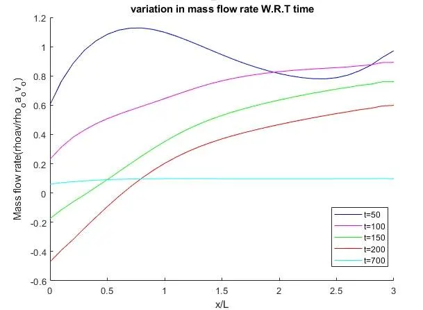
from the plot we can know that at lower time step mass flow rate is similar to sinosoidal and as the time steps increases the mass flow rate is becoming stable at time step 700 there is very slight change in the mass flow rate.

Plot showing properties at un steady state:

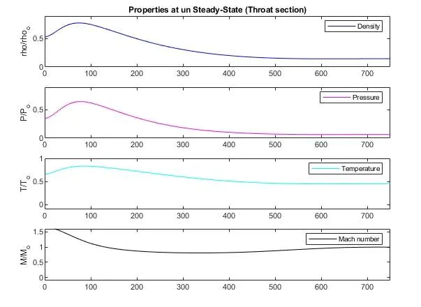
Its observed that the properties (temperature,massflowrate,pressure)at the throat are increased gradually and then continuously decreases till there is no change.But the mac number decreases and increases slightly.

Plot showing properties at steady state:

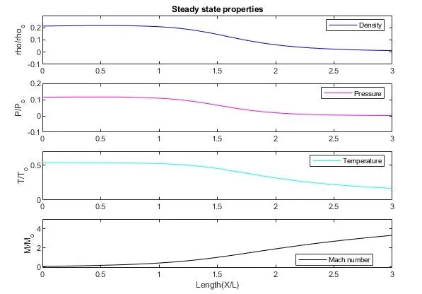
The properties (temperature,massflowrate,pressure) in a steady state is constant and gradually decreases.The mac number gradually increases.

Plot showing variation in mass-flow-rate with change in time step:

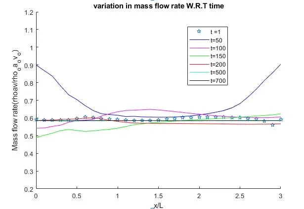
at start the mass flow rate is similar to constant and at 50 there is a increase and decrease and again increase takes place and at time step 700 it becomes constant (stable).

Plot showing properties at un steady state:

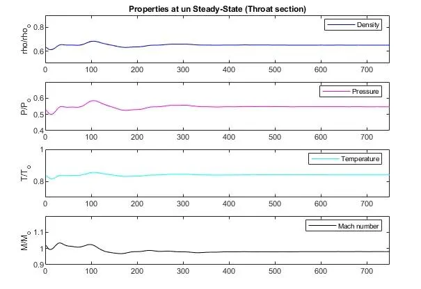
The properties (temperature,massflowrate,pressure) at throat section are very unstable untill 300 timesteps and becomes stable.

Plot showing properties at steady state:

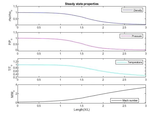
The properties (temperature,massflowrate,pressure) in a steady state is constant till 0.8 and gradually decreases.The mac number gradually increases.

Comparison of Normalized mass flow rate distributions of both forms

Grid Independence Test:

The grid independendace test is performed by changing no of grid points and observing how the results are changed.This test is performed to see whether the results change much or not.I have performed grid indepencenca test for 61 grid points and 31 .For the different grid size there is no large differences in the primitive variables like Mach number ratio,pressure ratio,temperature ratos ,density ratios .The differences are very small that they can be neglected.

Conclusion

• Simulation of non conservative form is easy and writing the code is also effort less.but the code for conservative form is large and more number of variables are present.
• The simulation time of non conservative form is less comparitively with conservative form.
• The errors in the non conservative form will be more because of more number of variables.
• Non conservative form attains stability soon compared to conservative form.
• The time steps in the conservative form is lesser than the time steps in the non conservative form.