Matlab code to animate the transient motion of a simple pendulum

Aim: Simulate the transient motion of simple pendulum solving ODE of motion of simple pendulum with damping.

Simple Pendulum: A bob or point mass attached to an un expandable string suspended from a fixed support is called simple pendulum.

periodic motion: A simple pendulum having a mass m hanging at alength l from the fixed pivot point when displaced at an angle the pendulum will swing to and fro with periodic motion.This motion will be opposed by damping.

Transient state: The state between starting of event and coming to steady state is called transient state.Simple pendulum exhibits transient behaviour .

Damping:Damping is the resistance to the motion within on or upon the system that has the influence in reducing or preventing the oscillations.Damping is some times wantedly induced into the system but often it is either should be reduced or removed.

Ode45: Ode45 is a predefined function in the matlab used for solving ODE’s. Ode45 is a function that solves ordinary or partial differential equations using a numerical method.

Ode45 can only solve first order derivatives . Therefore we must convert them to first order derivatives. The function ode45 takes 3 inputs. The 3 inputs are the function to be integrated, the time span and the initial conditions.

Equation for pendulum motion:

`(d^2 θ)/dt^2 +b/m (dθ)/ dt +g/l sin⁡θ=0`

g=acceleration due to gravity m/s2

l=length of the pendulum in m,(vertical length of string from center of bob to fixed position)

m=mass of the ball in kg,

d=damping coefficient

As this equation is in second order it need to be converte to first order differential equation.

`(dθ_1)/dt=θ_2`

`(dθ_2)/dt=(-bθ_2)/m-g/L sin⁡θ`

The euation is converted into first order differential equation

Initial Inputs:

l=1 m;

g=9.81 m/s2;

d=0.05;

m=1 k.g;

Matlab code:

Main code:

close all
clear all
clc
%solving ode using matlab
%inputs
b=0.05;    %damping coefficient
g=9.81;    %acceleration due to gravity
l=1;       %length of pendulum in meters
m=1 ;    %mass of the pendulum in kg
%initial condition
theta_0 = [0;3];%displacement and velocity(; used for getting column matrix)

%time
t_span = linspace(0,20,100);%command to get all values from 0-20 100 values

%solution to ode
[t,results]=ode45(@(t,theta)ode_function(t,theta,b,g,l,m),t_span,theta_0);
%store the output in t,results
%code to plot displacement and velocity wrt to time
figure(1)
plot(t,results(:,1))%plots the Displacement wrt time
hold on
plot (t,results(:,2))%plots the velocity wrt time
title('plot of displacement and velocity')%title to be displayed on graph
legend('displacement(rad)','velocity(rad/s)')%displays which line is for what
axis([0 20 -3 3])
xlabel('time')%x-axis name
ylabel ('plot')%y-axis name
grid on
%code to Animate motion of pendulum
z=1
for i=1:length(t_span)%repeats iteration length of t_span times
x_lap=l*sin(results(i,1));%stores all the x-co-ordinates
y_lap=-l*cos(results(i,1));%stores all the x-co-ordinates
x=0;
y=0;
figure(2)
plot([-2.5 2.5],[0 0],'g','linewidth',10)%plot for fixed beam
hold on%holds the structure
axis([-4 4 -2 0.5])%the graph position
plot([x x_lap],[y y_lap],'b','linewidth',5 )%All the values for the pendulum
plot(x_lap,y_lap,'o','markers',30,'markerfacecolor','r')%For bob 
title('Animation of motion of a pendulum')
xlabel('x-axis')
ylabel ('y-axis')
pause(0.05)%pause for each iteration
M(z)=getframe(gcf);%stores all the positions
hold off
z=z+1;%to get the images of all positions
%creating movie
end
movie(M);%create movie
video_pendulum=VideoWriter('pendulum Motion.avi')%
video_pendulum.FrameRate=4%sets frame rate to 10 
open(video_pendulum)
writeVideo(video_pendulum,M)%Writes video to M
close(video_pendulum)

Sub function:

Function to be called for solving ode:

function[dtheta_dt] = ode_function(t,theta,b,g,l,m)

      theta1 = theta(1);
      theta2=  theta(2);
      dtheta1_dt= theta2;
      dtheta2_dt= -(b/m)*theta2-(g/l)*sin(theta1);
      dtheta_dt= [dtheta1_dt; dtheta2_dt];
end      

Output:

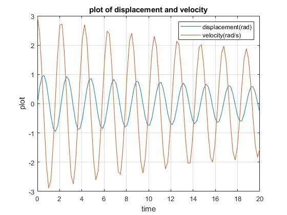
Results: 1.Graph showing displacement and velocity is plotted against time.

2.Animation video of pendulum motion is created .

Animation Video link: Animation of Simple Pendulum motion

Observation: When the velocity is zero the amplitude or displacement is maximum it is observed from the graph.

Conclusion:

1. Both the velocity and displacement from the neutral position will be reduced periodically as shown in the graph with respect to time.

Error occured:

Error correction:

changed the code to plot : plot([x x_lap],[y y_lap],'b','linewidth',5 )