Week 3 - Taylor table method and Matlab code

Aim: To compare Central ,skewed right scheme,skewe left scheme methods by solving a function and explaining the significance of them.we need to find second order derivative with fourth order approximation.

Function to be solved:

f = exp(x)*cos(x)

Procedure for taylors table method:

Approximate equation for skewed right hand method :

`( ∂ ^2 u) /(∂x^ 2) = af(i)+bf(i+1)+cf(i+2)+df(i+3)+ef(i+4)+gf(i+5)`

Approximate equation for skewed left hand method :

`( ∂ ^2 u) /(∂x^ 2) = af(i)+bf(i-1)+cf(i-2)+df(i-3)+ef(i-4)+gf(i-5)`

Approximate equation for Central method :

`( ∂ ^2 u) /(∂x^ 2) = af(i-2)+bf(i-1)+cf(i)+df(i+1)+ef(i+2)`

• The above approximations are expanded Deriving the 4th order approximations of the second-order derivativeand taylors table is filled.
• The series of equations got from the taylors table are solved by matrix inversion method.
• The equations are solved for the values of a,b,c,d,e,g. when we get all the values fo these coefficients,We solve the above mentioned approximations by substuting the values for a,b,c,d,e,g with the function as exp(x)*sin(x).

• %%Values for a,b,c,d,e,g for the approximation equations
  Skewed Right hand scheme =  
         15/4     
        -77/6     
        107/6     
        -13       
        61/12    
        -5/6 
  Skewed left hand scheme
       15/4     
       -77/6     
       107/6     
       -13       
        61/12    
        -5/6     
  Central difference scheme
        -1/12    
         4/3     
        -5/2     
         4/3     
        -1/12 
     

Taylors table for Skewed right hand difference scheme:

P - The order of accuracy

N - Number of nodes in the stencil N

Q - order of derivative

P = N + Q = 6

stensil	f(i)	f’(i)Δx	f’’(i)Δ^2	f’’’(i)Δ^3	f’’’’(i)Δ^4	f’’’'(i)Δ^5
af(i)	a	0	0	0	0	0
bf(i+1)	b	-b	/2	-1b/6	1b/24	-1b/120
cf(i+2)	c	-2c	2c	-8c/6	16c/24	-32c/120
df(i+3)	d	-3d	9d/2	-27d/6	81d/24	-243d/120
e(i+4)	e	-4e	8e	-64e/6	256e/24	-1024e/120
g(i+5)	g	-5g	25g/2	-125g/6	625g/24	-3125g/120

Taylors table for Skewed left hand difference scheme:

P = N + Q = 6

stensil	f(i)	f’(i)Δx	f’’(i)Δ^2	f’’’(i)Δ^3	f’’’’(i)Δ^4	f’’’'(i)Δ^5
af(i)	a	0	0	0	0	0
bf(i-1)	b	-b	/2	-1b/6	1b/24	-1b/120
cf(i-2)	c	-2c	2c	-8c/6	16c/24	-32c/120
df(i-3)	d	-3d	9d/2	-27d/6	81d/24	-243d/120
e(i-4)	e	-4e	8e	-64e/6	256e/24	-1024e/120
g(i-5)	g	-5g	25g/2	-125g/6	625g/24	-3125g/120

Taylors table for Central difference scheme:

P = N + Q - 1 = 5

stensil	f(i)	f’(i)Δx	f’’(i)Δ^2	f’’’(i)Δ^3	f’’’’(i)Δ^4
af(i-2)	a	-2a	2a	-8a/6	16a/24
bf(i-1)	b	-b	1b/2	-1b/6	1b/24
cf(i)	c	0	0	0	0
df(i+1)	d	d	d/2	d/6	d/24
e(i+2)	e	2e	4e/2	8e/6	16e/24

Matlab program:

Main program:

clear all
close all
clc
%initialization
x = pi/3;
dx = linspace(pi/4,pi/400,100);% linspace command produces specified 
%skewed right handed scheme
x_right = [ 1 1 1 1 1 1; 0 1 2 3 4 5;0 1/2 2 9/2 8 25/2;0 1/6 8/6 27/6 64/6 125/6;0 1/24 16/24 81/24 256/24 625/24;0 1/120 32/120 243/120 1024/120 3125/120]; 
y_right = [0;0;1;0;0;0];
format rat % returns values in fractions
z_right = inv(x_right)*y_right
%skewed left handed scheme
x_left = [ 1 1 1 1 1 1; 0 -1 -2 -3 -4 -5;0 1/2 2 9/2 8 25/2;0 -1/6 -8/6 -27/6 -64/6 -125/6;0 1/24 16/24 81/24 256/24 625/24;0 -1/120 -32/120 -243/120 -1024/120 -3125/120]; 
y_left = [0;0;1;0;0;0];
format rat
z_left = inv(x_left)*y_left
%skewed central method
x_central = [ 1 1 1 1 1; -2 -1 0 1 2; 2 1/2 0 1/2 2; -8/6 -1/6 0 1/6 8/6; 16/24 1/24 0 1/24 16/24];
y_central = [0;0;1;0;0];
format rat
z_central = inv(x_central)*y_central

%Calculation of error
for i=1:length(dx)
    Skewed_right_hand_difference_scheme_error(i) = Skewed_right_hand_difference_scheme(x,dx(i));
    Skewed_left_hand_difference_scheme_error(i)  =  Skewed_left_hand_difference_scheme(x,dx(i));
    central_difference_scheme_error(i)    =    Central_difference_scheme(x,dx(i));

end

figure(1)
loglog(dx,Skewed_right_hand_difference_scheme_error,'-ks','markers',5,'markerfacecolor','b','linewidth',1);
hold on
loglog(dx,Skewed_left_hand_difference_scheme_error,'marker','pentagram','markerfacecolor','b');
loglog(dx,central_difference_scheme_error,'-ko','markers',5,'markerfacecolor','y','linewidth',1);
xlabel('dx');
ylabel('errors in the schemes')
legend('Skewed right hand error','Skewed left hand error',' central error','location','best')
title('comparision of skewed right,skewed left and central scheme method')

sub programs:

Skewed right hand difference scheme:

%Skewed Right hand difference scheme
function out = Skewed_right_hand_difference_scheme(x,dx)
% analytical_solution
analytical_solution = -2*exp(x)*sin(x);
% Skewed_right_hand_difference_scheme
Skewed_right_hand_difference_scheme = ((15/4)*exp(x)*cos(x)-(77/6)*exp(x+dx)*cos(x+dx)+(107/6)*exp(x+2*dx)*cos(x+2*dx)-13.0000*exp(x+3*dx)*cos(x+3*dx)+ (61/12)*exp(x+4*dx)*cos(x+4*dx)-(5/6 )*exp(x+5*dx)*cos(x+5*dx))/dx^2;
% Skewed_right_hand_difference_scheme_error
out = abs(analytical_solution-Skewed_right_hand_difference_scheme);
end

Skewed left hand difference scheme:

%Skewed left hand difference scheme
function out = Skewed_left_hand_difference_scheme(x,dx)
% analytical_solution
analytical_solution = -2*exp(x)*sin(x);
% Skewed_leftt_hand_difference_scheme
Skewed_left_hand_difference_scheme = ((15/4)*exp(x)*cos(x)-(77/6)*exp(x-dx)*cos(x-dx)+(107/6)*exp(x-2*dx)*cos(x-2*dx)-13.0000*exp(x-3*dx)*cos(x-3*dx)+ (61/12)*exp(x-4*dx)*cos(x-4*dx)-(5/6)*exp(x-5*dx)*cos(x-5*dx))/dx^2;
% Skewed_left_hand_difference_scheme_error
out = abs(analytical_solution-Skewed_left_hand_difference_scheme);
end
         

Central difference scheme:

%Skewed Central difference scheme
function out = Skewed_Central_difference_scheme(x,dx)
% analytical_ second order solution
analytical_solution = -2*exp(x)*sin(x);
% Skewed_Central_difference_scheme
Skewed_Central_difference_scheme = ((-1/12)*exp(x-2*dx)*cos(x-2*dx)+(4/3)*exp(x-dx)*cos(x-dx)-(5/2)*exp(x)*cos(x)+(4/3 )*exp(x+dx)*cos(x+dx)-(1/12)*exp(x+2*dx)*cos(x+2*dx))/dx^2;
%Skewed_Central_difference_scheme_error
out = abs(analytical_solution-Skewed_Central_difference_scheme);
end

Code Explaination:

1. Initialization of values for dx and x ,linspace command is used for the initialization of the dx values.
2. the coefficiens we got from the expansion of the approximate equations are made into matrix form AX = B.
3. By using the inversion method (z_right = inv(x_right)*y_right)we solve for the variables a,b,c,d,e and g.
4. three subfunctions are written to be called for skewed right hand, skewed left hand and central scheme with the formulas for analytical deivative for second order in each function.
5. The sub functions are written to give the absolute difference between theanalytical value and the schemes.
6. For loop is used in the main program to get the values of the Central difference,right hand and left hand scheme for a set of x values.
7. Plots are made with entral difference,right hand and left hand scheme values aginst dx .

Plots comparing errors among schemes:

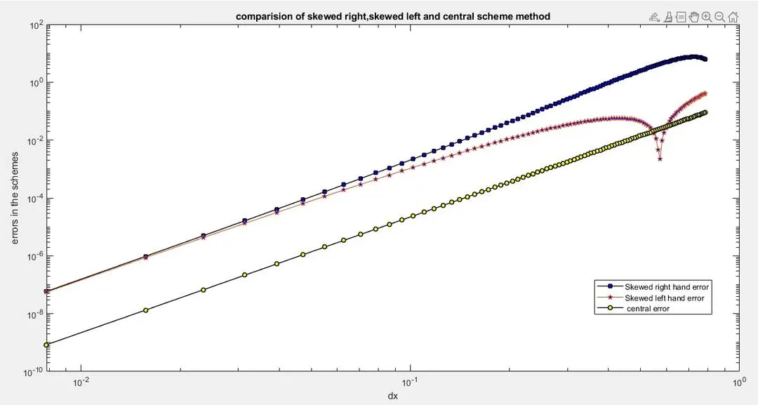
Conclusions from graph:

1. Central difference scheme has the least error among the three schemes.
2. Skewed left hand scheme and schewed right hand scheme both has the same error at the start and after few points the error in the skewed left hand scheme shows considerably high reduction and then comes to its previous range.
3. The slope of central difference scheme seems to be same throughout the plot.
4. the slope of skewed right hand scheme aloso appears to be same but the re is slight negative slope at the end.
5. the slope of the left skewed scheme is not the same throughout.

How a skewed scheme is useful? What can a skewed scheme do that a CD scheme cannot?

• Central difference scheme computation time is comparitively less. error in this scheme is also very less.
• Central difference scheme cant be solved when boundary conditions are defined.when higher orders are to be solved we use skewed schemes,when we know atleast one boundary we can use skewed schemes to solve them.