Linear, CubicFit & SplitWise method using matlab

Aim: To write code to fit a linear and cubic polynomial for the Cp data and to write a code for splitwise method using matlab.

Curve fit: It is a process of constructing a curve or mathematical function which have the closest proximity to the history of data.It helps in oredicting the outcomes without actually conducting the experiment.This is very helpful in predicting natural processes .Fitted curves can be used as data visuvalization.We can generate an equation for the data we have.It is possible to represent the patterns for the data.

Original data:

%Original data
clear all 
close all
clc
%Getting data
cp_data = load('data');%load is used to get the data into matlab
%assigning data
Temperature = cp_data(:,1);
cp = cp_data(:,2);
plot(Temperature,cp,'linewidth',3)
xlabel('Temperature[k]');
ylabel('Specific heat [KJ/kmol-k]')

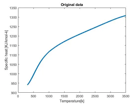
Plot showing original data:

Linear polynomial : curve fit using first order polynomial.This will not pass through all the data points .It is the least accurate order in the curve fit.

%curve fit
clear all 
close all
clc
%Getting data
cp_data = load('data');
%assigning data
Temperature = cp_data(:,1);
cp = cp_data(:,2);
%Predicting cp
co_effi = polyfit(Temperature,cp,1);%gives co-efficients for given order
predicted_cp = polyval(co_effi,Temperature);%calculates cp for calculated co-efficients
%comparing curve fit with original data
figure
plot(Temperature,cp,'linewidth',3,'color','b');
hold on
plot(Temperature,predicted_cp,'linewidth',3,'color','r');
xlabel('Temperature[k]');
ylabel('Specific heat [KJ/kmol-k]')
legend('original dataset','curve fit','location','southeast')
title('Linear curve')
hold off

Plot comparing original data with Predicted data(Linear curve):

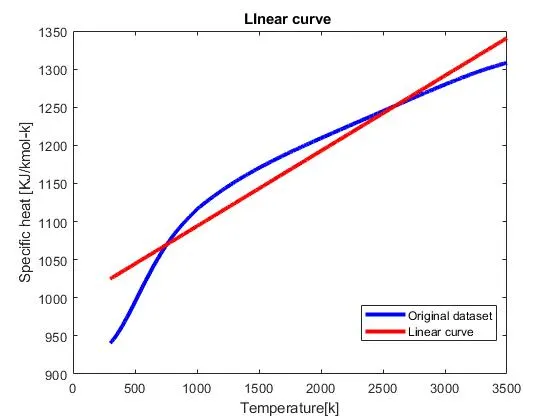
Linear curve barely passes through all the given data points.In order to get good fit we need to increase order.

Cubic polynomial :

[p,s,mu] = polyfit(x,y,n) also returns mu, which is a two-element vector with centering and scaling values. mu(1) is mean(x), and mu(2) is std(x). Using these values, polyfitcenters x at zero and scales it to have unit standard deviation,

This centering and scaling transformation improves the numerical properties of both the polynomial and the fitting algorithm.

%cubic Fit
clear all 
close all
clc
%Getting data
cp_data = load('data');
%assigning data
Temperature = cp_data(:,1);
cp = cp_data(:,2);
[co_effi,s,mu] = polyfit(Temperature,cp,3);%gives co-efficients for given order along with mu and s.mu contains mean and standard deviation ,s returns structure
predicted_cp = polyval(co_effi,Temperature,s,mu);%calculates cp for calculated co-efficients
%Goodness of fit
 error = predicted_cp -cp ;
 sse = sum(error.^2);
 ssr = sum((cp- mean(cp)).^2);
 sst = ssr + sse;
 R_square= (ssr)/(sst);
 if R_square >0.95 
     display('good Fit');
 else
     display('bad Fit');
 end
%plotting
plot(Temperature,cp,'linewidth',3,'color','b');
hold on
plot(Temperature,predicted_cp,'linewidth',3,'color','r');
xlabel('Temperature[k]');
ylabel('Specific heat [KJ/kmol-k]')
title('Cubic curve')
legend('original dataset','curve fit','location','southeast')
hold off

Plot comparing original data and curve fit data using cubic curve:

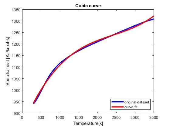
Cubic curve apperas to be closer to the original data curve.

Splitwise Method:

In this method data is splitted into parts and curve fitting procedure is applied.This method gives fit that accurately fits with the data curve.but it needs a bit longer code to perform this method.

%Splitwise Method
clear all
close all 
clc
%Getting data
cp_data = load('data');
%assigning data
Temperature = cp_data(:,1);
cp = cp_data(:,2);
%splitting data
temp1 = cp_data(1:500,1);
cp1 = cp_data(1:500,2);

temp2 = cp_data(501:1000,1);
cp2 = cp_data(501:1000,2);

temp3 = cp_data(1001:1500,1);
cp3 = cp_data(1001:1500,2);

temp4 = cp_data(1501:2000,1);
cp4 = cp_data(1501:2000,2);

temp5 = cp_data(2001:2500,1);
cp5 = cp_data(2001:2500,2);

temp6 = cp_data(2501:3000,1);
cp6 = cp_data(2501:3000,2);

temp7 = cp_data(3001:3200,1);
cp7 = cp_data(3001:3200,2);

[co_effi1,s1,mu1] = polyfit(temp1,cp1,3);
predicted_cp1 = polyval(co_effi1,temp1,s1,mu1);
[co_effi2,s2,mu2] = polyfit(temp2,cp2,3);
predicted_cp2 = polyval(co_effi2,temp2,s2,mu2);
[co_effi3,s3,mu3] = polyfit(temp3,cp3,3);
predicted_cp3 = polyval(co_effi3,temp3,s3,mu3);
[co_effi4,s4,mu4] = polyfit(temp4,cp4,3);
predicted_cp4 = polyval(co_effi4,temp4,s4,mu4);
[co_effi5,s5,mu5] = polyfit(temp5,cp5,3);
predicted_cp5 = polyval(co_effi5,temp5,s5,mu5);
[co_effi6,s6,mu6] = polyfit(temp6,cp6,3);
predicted_cp6 = polyval(co_effi6,temp6,s6,mu6);
[co_effi7,s7,mu7] = polyfit(temp7,cp7,3);
predicted_cp7 = polyval(co_effi7,temp7,s7,mu7);
%ploting 
plot(Temperature,cp,'linewidth',5,'color','g');
hold on
plot(temp1,predicted_cp1,'linewidth',1,'color','b');
plot(temp2,predicted_cp2,'linewidth',1,'color','b');
plot(temp3,predicted_cp3,'linewidth',1,'color','b');
plot(temp4,predicted_cp4,'linewidth',1,'color','b');
plot(temp5,predicted_cp5,'linewidth',1,'color','b');
plot(temp6,predicted_cp6,'linewidth',1,'color','b');
plot(temp7,predicted_cp7,'linewidth',1,'color','b');
hold off
xlabel('Temperature[k]');
ylabel('Specific heat [KJ/kmol-k]')
title('Cubic curve using Splitwise method ')
legend('original dataset','curve fit','location','southeast')

Plot for the cubic curve using Splitwise Method:

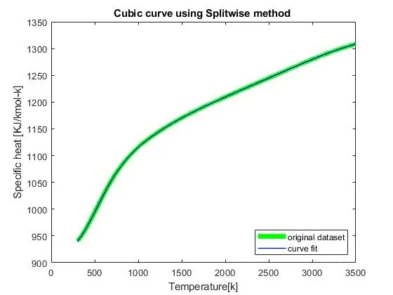
SplitWise method makes the curve fit a perfect fit as every point in curve fit coinsides with the original data.

SplitWise code explaination:

1. Getting the data from the file to the matlab using 'load' command.It is important to see that the file need to be used should be inthe same location as the code.
2. Assigning the data to cp_data,then Assigning the Data to Temperature and cp {(Temperature = cp_data(:,1)),cp = cp_data(:,2)}.
3. splitting the data by assigning part of data to some different variable names with numbers.Data is splitted into 7 parts.
4. Using polyfit command is used to find the coefficients of the polynomial,then assigning them to co-effi.
5. Using polyval command to calculate the cp values {predicted_cp1 = polyval(co_effi1,temp1,s1,mu1)}.The explaination for mu and su is given above.
6. Plotting the original data and Curvefit data curves.

Evaluation of Goodness of fit: After fitting the data with one or more models Goodness of Fit must be evaluated. you should examine the goodness of fit statistics. There are few methods to evaluate the goodness of fit. you should examine the goodness of fit statistics. The Curve Fitting Toolbox supports these goodness of fit statistics for parametric models:

• The sum of squares due to error (SSE)
• R-square {R-square can take on any value between 0 and 1, with a value closer to 1 indicating a better fit}
• Adjusted R-square {The adjusted R-square statistic can take on any value less than or equal to 1, with a value closer to 1 indicating a better fit}
• Root mean squared error (RMSE) {A RMSE value closer to 0 indicates a better fit}

Error = |y(i) - f(x(i))|

SSE =`sum_(i=1)^n`Error`(i)^2`

`R^2`=`(SSR)/(SST)`

SST = SSR + SSE

RSME = `root()((SSE)/n)` n = Total number of data points

Using curve Fitting Tool to evaluate the fit:

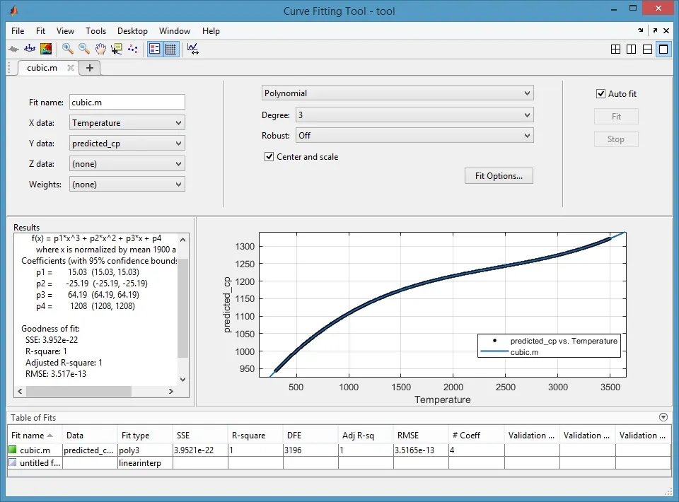
1. Ways to get Perfect Fit: Fit in which the predicted curve exactly fits the original data curve with no errors is called PerfectFit .We can get the perfect curve either by increasing the order or by using ths splitWise method as shown above.If there are n points you can fit polynomials of (n-1) degree to exactly pass through points.
2. Ways to get Best Fit: For a curve to be a BestFit it should have least sum of squares,if the R^2 value is 1 then it is called the BestFit.
3. Method to improve CubicFit: The cubicFit can be improved by using Splitwise method to eliminate the deviation from the original curve.

References: MathWorks Help center, Skill lynk Projects,wikipedia ,Math.uah.edu