Week 7 - Simulation of a 1D Super-sonic nozzle flow simulation using Macormack Method
STUDY ON QUASI 1D SUBSONIC-SUPERSONIC
ISENTROPIC NOZZLE FLOW
AIM:
To study the Conservation and Non-Conservation form of the governing equations of quasi 1D convergent-divergent nozzle flow using the MacCormack’s method of discretization.
GOVERNING EQUATION:
- Conservative form of governing equation:
- Continuity Equation:
`del(rhoA)//delt+del(rhoAv)//delx = 0`
- Momentum Equation:
`del(rhoAv)//delt+del(rhoAv^2)//delx = -AdelP//delx`
- Energy Equation:
`del(rhoAv^2/2)//delt+del(rhoAv^3/2)//delx = -AvdelP//delx`
General representation of these equations is `del(phi)//delt+del(phiv)//delx = R.H.S`.
- Non-Conservative form of governing equation:
- Continuity Equation:
`delrho//delt = -rhodelv//delx-rhovdel(lnA)//delx-vdelrho//delx`
- Momentum Equation:
`delv//delt = -vdelv//delx-(1/gamma)(delT//delx+T/rho(delrho//delx))`
- Energy Equation:
`delT//delt = -vdelT//delx-(gamma-1)T(delv//delx+v(del(lnA)//delx))`
Note that all the above governing equations are in the non-dimensional form in order to code for the respective solutions.
THEORY:
MacCormack’s Technique:
The MacCormack method is a widely used discretization scheme in CFD for obtaining the numerical of non-linear hyperbolic partial differential equations. Since this method is 2nd order accurate in both space and time, it is comparatively more accurate than forward, rearward or even upwind scheme and is preferred for solving most non-linear CFD problems. In this technique, we implement 2 steps namely; (i) Predictor Step & (ii) Corrector Step.
In the Predictor step, using the initial conditions of the governing equations, we solve for the time derivative, ` (delf//delt)_p `, where ‘f’ is any parametric variable, by using Forward Differencing Scheme.
With the computation of the predictor step, we are going to calculate for the intermediate Solution update given by Taylor series as `f' = f_(Initial) + ((delf)/(delt))_p.Deltat`.
In the Corrector step, we implement the updated value of `f’` to determine the time derivative, `(delf//delt)_c `, by using Backward Differencing Scheme.
Finally, we calculate the average time derivative of the predictor and corrector steps, `((delf)/(delt))_(avg) = 0.5[((delf)/(delt))_p+((delf)/(delt))_c]`.
Using `((delf)/(delt))_(avg)`, we calculate the final solution update for ‘f’ using the initial value of ‘f’ for this time step, `f = f_(Initial) + ((delf)/(delt))_(avg).Deltat`.
The only difference between the predictor and the corrector step is that, for predictor step, we use forward scheme and for corrector step, we use backward scheme for the space derivatives.
Initial & Boundary Conditions:
The initial conditions used for finding the primitive variables using MacCormack technique is given by;
- For Non-conservative form of the governing equation:
`rho = 1-0.3146x`
`T = 1-0.2314x`
`v = (0.1+1.09x)T^(1/2)`
`A = 1+2.2(x-1.5)^2 in 0<=x<=3`
Where `rho` is the density of fluid flowing through the nozzle
`T` is the temperature of the fluid
`v` is the velocity of the fluid
`A` is the area profile of the nozzle
`x` is the distance of all the grid points from inlet to outlet of nozzle
- For Conservative form of the governing equation:
`rho = 1, T = 1 in 0<=x<=0.5`
`rho = 1-0.366(x-0.5), T = 1-0.167(x-0.5) in 0.5<=x<=1.5`
`rho = 0.634-0.3879(x-1.5), T = 0.833-0.3507(x-1.5) in 1.5<=x<=3.5`
` A = 1+2.2(x-1.5)^2 in 0<=x<=3`
`v = 0.59/(rhoA)`
Note that the primitive variables shown above are in non-dimensional form since the governing equations are also in the non-dimensional form.
The boundary conditions at the subsonic inflow boundary, we must fix or specify the values of two dependent flow-field variables, whereas the value of one other variable must be allowed to float. The flow-field variable that is allowed to float in our case is the velocity, v, while the density and temperature are fixed, since the left-running characteristics is in the upstream direction while the right-running characteristics travel downstream at the inlet. The boundary condition at the supersonic outflow boundary, we float all the independent flow-field variables since both the left-running and right-running characteristics are downstream towards the right side of the flow.
Therefore, for non-conservative form, at inlet, by using linear extrapolation between two internal points,
`v_1 = 2v_2-v_3`
At outlet,
`v_n = 2v_(n-1)-v_(n-2)`
`rho_n = 2rho_(n-1)-rho_(n-2)`
`T_n = 2T_(n-1)-T_(n-2)`
For conservative form at inlet and outlet, we introduce 2 terms ‘U’ and ‘F’ for solving the governing equations. These terms are a function of the primitive variables which can be used to solve the governing equations and to find those primitive variables.
In the conservative form of the governing equations, the time derivative terms are considered to be ‘U’ and space derivative terms are considered to be ‘F’ and is called as the ‘Flux’ terms.
`U_1 = rhoA; U_2 = rhoAv; U_3 = rhoA(T/(gamma-1) + 0.5gammav^2)`
‘F’ can be written as a function of primitive variables but as we progress on with our coding part, we will face stability problem even if the courant number is less than 0.5. This is because of the dependent variables which occur explicitly are the U1, U2 and U3 and not the primitive variables causing lack of purity in the flux terms. So, ‘F’ is coded in terms of ‘U’, i.e.,
`F_1 = F_1(U_1, U_2, U_3)`
`F_1 = F_2(U_1, U_2, U_3)`
`F_1 = F_3(U_1, U_2, U_3)`
`J_2 = J(U_1,U_2,U_3)`
And the respective equations after derivation are,
`F_1 = U_2`
`F_2 = U_2^2/U_1+(gamma-1)/gamma(U_3-(gamma)/(2)(U_2^2/U_1))`
`F_3 = gamma(U_2U_3)/U_1-(gamma(gamma-1))/2U_2^3/U_1^2`
`J_2 = (gamma-1)/gamma(U_3-(gamma)/(2)(U_2^2/U_1))del(lnA)//delx`
Where `J_2` is the additional term present on the RHS of the Conservation form of the Momentum equation.
So, for the time steps, the boundary conditions applied for the Conservation form of the governing equations are, just like the non-conservation form, at the inlet, velocity is floated while temperature and density are fixed, in our case the initial condition `rho_1 = 1, T_1 = 1`, so, Inflow BCs are,
`(U_1)_1 = rho_1A_1 = A_1`
`(U_2)_1 = 2(U_2)_2 – (U_2)_3`
`(U_3)_1 = (U_1)_1(T_1/(gamma-1)+gamma/2v_1^2)`
The Outflow BCs are,
`(U_1)_n = 2(U_1)_(n-1) – (U_1)_(n-2)`
`(U_2)_n = 2(U_2)_(n-1) – (U_2)_(n-2)`
`(U_3)_n = 2(U_3)_(n-1) – (U_3)_(n-2)`
Similarly, the Flux variables and the primitive variables at the outlet can be determined.
PROCEDURE:
- This whole study program is coded and simulated using Matlab Software.
- For grid independence, I chose the accuracy of my solution to be 99% and above. So, for coding, I used n = 61 grid points which gave me results with error less than 1%.
-
% Program for Quasi 1D Convergent-Divergent Nozzle Flow Equation clear all; close all; clc; %Inputs n = 61;% number of grid points x = linspace(0,3,n);% total distance of the domain split into n grid points dx = x(2)-x(1); nt = 1400;% number of time steps dt = 0.01; gamma = 1.4;% ratio of specific heats % Initial conditions for Non-conservative form of the quasi 1D nozzle flow % Every parameter used in this calculation is non-dimensionalized rho = 1-0.3146.*x;% Non-dimensional Density T = 1-0.2314.*x;% Non-dimensional Temperature v = (0.1+1.09.*x).*T.^0.5;% Non-dimensional Velocity A = 1+2.2*(x-1.5).^2;% Non-dimensional Area % Function call for Non-conservation form of the governing equations [rho_nc, T_nc, v_nc, m_nc] = non_conservation_1d_nozzle_flow(x,n,dx,nt,dt,gamma,rho,T,v,A); % Function call for Conservation form of the governing equations [rho_c, T_c, v_c, m_c] = conservation_1d_nozzle_flow(x,n,nt,gamma,A); %Plot for mass flow distribution comparison of both forms figure(7) plot(x,m_nc(end,:),'linewidth',3,'color','b'); hold on; plot(x,m_c(end,:),'linewidth',3,'color','r'); xlabel('Non-dimensional distance through the nozzle, x'); ylabel('Mass flow rate, m'); axis([0 3 0.58 0.589]); title('Comparison of normalized Mass flow rate of both forms'); legend('Non-Conservation Form','Conservation form'); - In the above main program, the major inputs used by both the forms of governing equation are defined. The initial conditions for the non-conservative form are defined and the function call for non-conservative and conservative forms are done with separate function calls and results. These results obtained are then used to plot the normalized mass flow rate comparison between both the forms which is one of the expected results.
-
% Function for Non-conservative form of the quasi 1D nozzle flow equations function [rho, T, v, m] = non_conservation_1d_nozzle_flow(x,n,dx,nt,dt,gamma,rho,T,v,A) q = 1;% loop counter initialization for k=1:nt % Initializing old values in variable for later use rho_old = rho; T_old = T; v_old = v; % Predictor method or step for i = 2:n-1 % Major terms in the equation drho_dx = (rho(i+1)-rho(i))/dx; dv_dx = (v(i+1)-v(i))/dx; dT_dx = (T(i+1)-T(i))/dx; dlnA_dx = (log(A(i+1))-log(A(i)))/dx; % Continuity equation drho_dt_p(i) = -rho(i)*dv_dx -rho(i)*v(i)*dlnA_dx -v(i)*drho_dx; % Momentum equation dv_dt_p(i) = -v(i)*dv_dx -(1/gamma)*(dT_dx + (T(i)/rho(i))*drho_dx); % Energy equation dT_dt_p(i) = -v(i)*dT_dx -(gamma-1)*T(i)*(dv_dx +v(i)*dlnA_dx); % Solution update for Predictor step rho(i) = rho(i) + drho_dt_p(i)*dt; v(i) = v(i) + dv_dt_p(i)*dt; T(i) = T(i) + dT_dt_p(i)*dt; end % Corrector method or step for i = 2:n-1 % Major terms in the equation drho_dx = (rho(i)-rho(i-1))/dx; dv_dx = (v(i)-v(i-1))/dx; dT_dx = (T(i)-T(i-1))/dx; dlnA_dx = (log(A(i))-log(A(i-1)))/dx; % Continuity equation drho_dt_c(i) = -rho(i)*dv_dx -rho(i)*v(i)*dlnA_dx -v(i)*drho_dx; % Momentum equation dv_dt_c(i) = -v(i)*dv_dx -(1/gamma)*(dT_dx + (T(i)/rho(i))*drho_dx); % Energy equation dT_dt_c(i) = -v(i)*dT_dx -(gamma-1)*T(i)*(dv_dx +v(i)*dlnA_dx); end % Computing average time derivative drho_dt_avg = 0.5*(drho_dt_p + drho_dt_c); dv_dt_avg = 0.5*(dv_dt_p + dv_dt_c); dT_dt_avg = 0.5*(dT_dt_p + dT_dt_c); for j=2:n-1 % Final solution update rho(j) = rho_old(j) + drho_dt_avg(j)*dt; v(j) = v_old(j) + dv_dt_avg(j)*dt; T(j) = T_old(j) + dT_dt_avg(j)*dt; end % Apply Boundary conditions % At inlet v(1) = 2*v(2)-v(3); % At outlet v(n) = 2*v(n-1) -v(n-2); rho(n) = 2*rho(n-1) -rho(n-2); T(n) = 2*T(n-1) -T(n-2); % Plot for timewise variation of primitive variables figure(1) subplot(3,1,1); title('Timewise variation of primitive varaibles at grid point i=31'); hold on; plot(k,rho(31),'.','linewidth',3,'color','b'); xlabel('Time-step, nt'); ylabel('Non-dimensional density, rho'); hold off; subplot(3,1,2); hold on; plot(k,T(31),'.','linewidth',3,'color','r'); xlabel('Time-step, nt'); ylabel('Non-dimensional Temperature, T'); hold off; subplot(3,1,3); hold on; plot(k,v(31),'.','linewidth',3,'color','g'); xlabel('Time-step, nt'); ylabel('Non-dimensional velocity, v'); hold off; % Plot for Steady state distribution of primitive variables if k==1400 figure(2) subplot(3,1,1) plot(x,rho,'linewidth',3,'color','b'); ylabel('Non-dimensional density, rho'); xlabel('Non-dimensional distance through the nozzle, x'); title('Steady state distribution of primitive variables inside the nozzle'); subplot(3,1,2) plot(x,T,'linewidth',3,'color','r'); ylabel('Non-dimensional Temperature, T'); xlabel('Non-dimensional distance through the nozzle, x'); subplot(3,1,3) plot(x,v,'linewidth',3,'color','g'); ylabel('Non-dimensional velocity, v'); xlabel('Non-dimensional distance through the nozzle, x'); end % Plot for mass flow rate distribution of primitive variables if k==1||k==50||k==100||k==250||k==500||k==700||k==1400 m(q,:) = rho.*A.*v;% use of loop counter 'q' figure(3) hold on; txt = sprintf('%d th Time-step',k); plot(x,m(q,:),'linewidth',2,'DisplayName',txt); xlabel('Non-dimensional distance through the nozzle, x'); ylabel('Mass flow rate, m'); title('Mass flow rate distribution inside the nozzle at different Time-steps'); hold off; legend; q = q+1; end end end - In the first function program, which is the Non-conservative form, the time loop followed by the space loop for the Predictor method is defined. After the predictor step, the solution update for the predictor step is given which is then taken as the input for the Corrector method. Ones both the time derivatives for the Predictor and Corrector method are ready, we determine the average time derivative for the final solution update. This is the completion of one time step, this whole process is repeated inside the time loop until a steady solution is reached. Before the next time step, we need to initialize the BCs for inlet and outlet of the nozzle. The plot command is used to represent the results in a graphical manner for comparison.
-
% Function for Conservative form of the quasi 1D nozzle flow equations function [rho, T, v, m] = conservation_1d_nozzle_flow(x,n,nt,gamma,A) q = 1;% loop counter initializing % Initializing conservative form Initial conditions for i=1:n if x(i)>=0&&x(i)<=0.5 rho(i) = 1; T(i) = 1; elseif x(i)>=0.5&&x(i)<=1.5 rho(i) = 1-0.366*(x(i)-0.5); T(i) = 1-0.167*(x(i)-0.5); elseif x(i)>=1.5&&x(i)<=3.5 rho(i) = 0.634-(0.3879*(x(i)-1.5)); T(i) = 0.833-(0.3507*(x(i)-1.5)); else break end end v = 0.59./(rho.*A); % Initial condition for the function parameters u1 = rho.*A; u2 = rho.*A.*v; u3 = rho.*A.*((T./(gamma-1))+0.5*gamma.*v.^2); dx = x(end)/(n-1); dt = 0.01; for k=1:nt % Time-wise initial conditions u1_old = u1; u2_old = u2; u3_old = u3; % Initial condition for flux parameters f1 = u2; f2 = (u2.^2./u1)+((gamma-1)/gamma)*(u3-(0.5*gamma.*u2.^2./u1)); f3 = (gamma.*u2.*u3./u1)-(0.5*gamma*(gamma-1).*u2.^3./u1.^2); % Predictor method or step for i = 2:n-1 % Major terms in the equation df1_dx = (f1(i+1)-f1(i))/dx; df2_dx = (f2(i+1)-f2(i))/dx; df3_dx = (f3(i+1)-f3(i))/dx; j2 = (1/gamma)*rho(i)*T(i)*((A(i+1)-A(i))/dx); du1_dt_p(i) = -df1_dx; du2_dt_p(i) = -df2_dx + j2; du3_dt_p(i) = -df3_dx; % Solution update for Predictor step u1(i) = u1(i) + du1_dt_p(i)*dt; u2(i) = u2(i) + du2_dt_p(i)*dt; u3(i) = u3(i) + du3_dt_p(i)*dt; % Solution update for flux variables f1(i) = u2(i); f2(i) = (u2(i)^2/u1(i))+(((gamma-1)/gamma)*(u3(i)-(0.5*gamma*u2(i)^2/u1(i)))); f3(i) = (gamma*u2(i)*u3(i)/u1(i))-(0.5*gamma*(gamma-1)*u2(i)^3/u1(i)^2); %Solution update for primitive variables rho(i) = u1(i)/A(i); T(i) = (gamma-1)*((u3(i)/u1(i))-(0.5*gamma*(u2(i)/u1(i))^2)); end % Corrector method or step for i = 2:n-1 % Major terms in the equation df1_dx = (f1(i)-f1(i-1))/dx; df2_dx = (f2(i)-f2(i-1))/dx; df3_dx = (f3(i)-f3(i-1))/dx; j2 = (1/gamma)*rho(i)*T(i)*((A(i)-A(i-1))/dx); du1_dt_c(i) = -df1_dx; du2_dt_c(i) = -df2_dx+j2; du3_dt_c(i) = -df3_dx; end % Computing average time derivative du1_dt_avg = 0.5*(du1_dt_p+du1_dt_c); du2_dt_avg = 0.5*(du2_dt_p+du2_dt_c); du3_dt_avg = 0.5*(du3_dt_p+du3_dt_c); for j=2:n-1 % Final solution update u1(j) = u1_old(j) + du1_dt_avg(j)*dt; u2(j) = u2_old(j) + du2_dt_avg(j)*dt; u3(j) = u3_old(j) + du3_dt_avg(j)*dt; rho(j) = u1(j)/A(j); v(j) = u2(j)/u1(j); T(j) = (gamma-1)*((u3(j)/u1(j))-0.5*gamma*v(j)^2); end % Apply Boundary conditions % At inlet u1(1) = rho(1)*A(1); u2(1) = 2*u2(2)-u2(3); v(1) = u2(1)/u1(1); u3(1) = u1(1)*((T(1)/(gamma-1))+0.5*gamma*v(1)^2); % At outlet u1(n) = 2*u1(n-1)-u1(n-2); u2(n) = 2*u2(n-1)-u2(n-2); u3(n) = 2*u3(n-1)-u3(n-2); f1(n) = u2(n); f2(n) = (u2(n)^2/u1(n))+((gamma-1)/gamma)*(u3(n)-(0.5*gamma*u2(n)^2/u1(n))); f3(n) = (gamma*u2(n)*u3(n)/u1(n))-(0.5*gamma*(gamma-1)*u2(n)^3/u1(n)^2); rho(n) = u1(n)/A(n); v(n) = u2(n)/u1(n); T(n) = (gamma-1)*((u3(n)/u1(n))-0.5*gamma*v(n)^2); % Plot for timewise variation of primitive variables figure(4) subplot(3,1,1); title('Timewise variation of primitive varaibles at grid point i=31(Conservative Form)'); hold on; plot(k,rho(31),'.','linewidth',3,'color','b'); xlabel('Time-step, nt'); ylabel('Non-dimensional density, rho'); hold off; subplot(3,1,2); hold on; plot(k,T(31),'.','linewidth',3,'color','r'); xlabel('Time-step, nt'); ylabel('Non-dimensional Temperature, T'); hold off; subplot(3,1,3); hold on; plot(k,v(31),'.','linewidth',3,'color','g'); xlabel('Time-step, nt'); ylabel('Non-dimensional velocity, v'); hold off; % Plot for Steady state distribution of primitive variables if k==1400 figure(5) subplot(3,1,1) plot(x,rho,'linewidth',3,'color','b'); ylabel('Non-dimensional density, rho'); xlabel('Non-dimensional distance through the nozzle, x'); title('Steady state distribution of primitive variables inside the nozzle(Conservative Form)'); subplot(3,1,2) plot(x,T,'linewidth',3,'color','r'); ylabel('Non-dimensional Temperature, T'); xlabel('Non-dimensional distance through the nozzle, x'); subplot(3,1,3) plot(x,v,'linewidth',3,'color','g'); ylabel('Non-dimensional velocity, v'); xlabel('Non-dimensional distance through the nozzle, x'); end % Plot for mass flow rate distribution of primitive variables if k==1||k==50||k==100||k==250||k==500||k==700||k==1400 m(q,:) = rho.*A.*v; figure(6) hold on; txt = sprintf('%d th Time-step',k); plot(x,m(q,:),'linewidth',2,'DisplayName',txt); xlabel('Non-dimensional distance through the nozzle, x'); ylabel('Mass flow rate, m'); title('Mass flow rate distribution inside the nozzle at different Time-steps(Conservative Form)'); hold off; legend; q = q+1; end end end - In the second function program, which is the Conservative form, the initial conditions are determined for the Flux variables which are used in the governing equations. The same steps are done for the conservative form as in the non-conservative form. The only difference is that we need to derive the primitive variables from the function ‘U’ terms and also use the flux terms must be calculated at the boundaries since they are needed in the predictor step.
RESULTS:
Thus the study on Conservation and Non-Conservation form of the governing equations of quasi 1D convergent-divergent nozzle flow using the MacCormack’s method of discretization is successfully conducted and the respective plots are plotted using the Matlab software.
(i) Timewise variation of primitive variables:
Non-Conservation Form (n = 31 & n = 61):
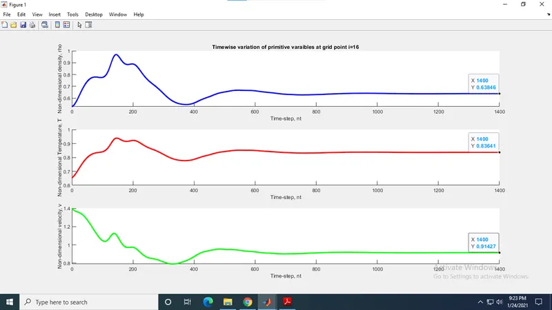
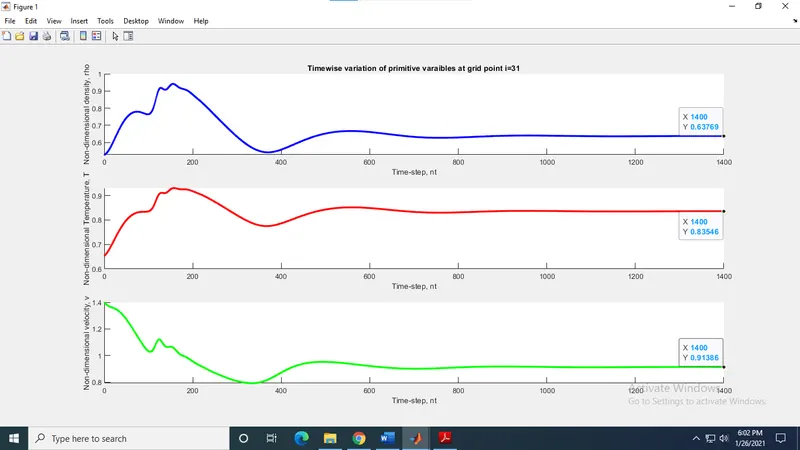
Conservation Form (n = 31 & n = 61):
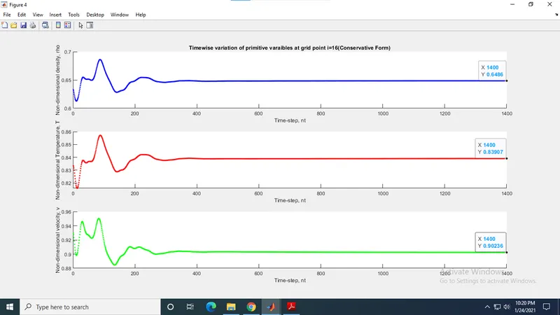
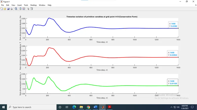
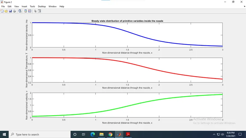
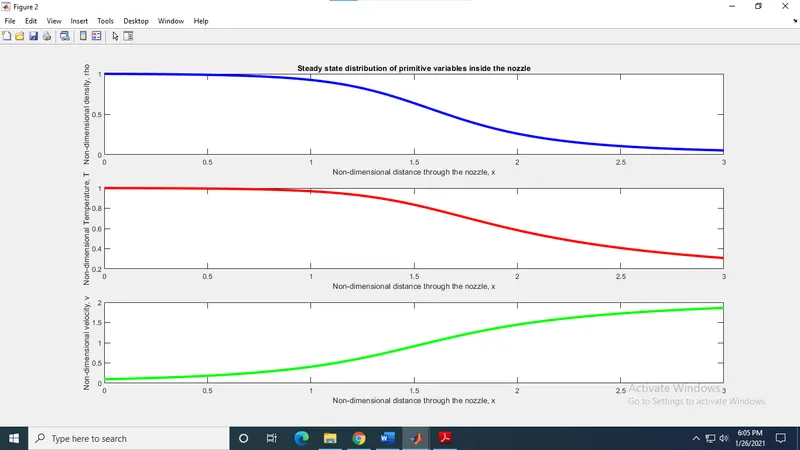
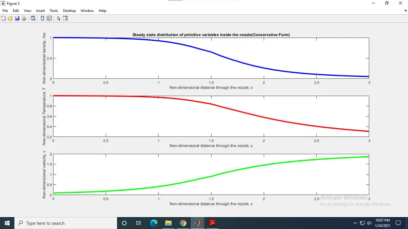
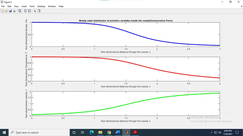
(ii) Steady state distribution of primitive variables:
Non-Conservation Form (n = 31 & n = 61):
Conservation Form (n = 31 & n = 61):
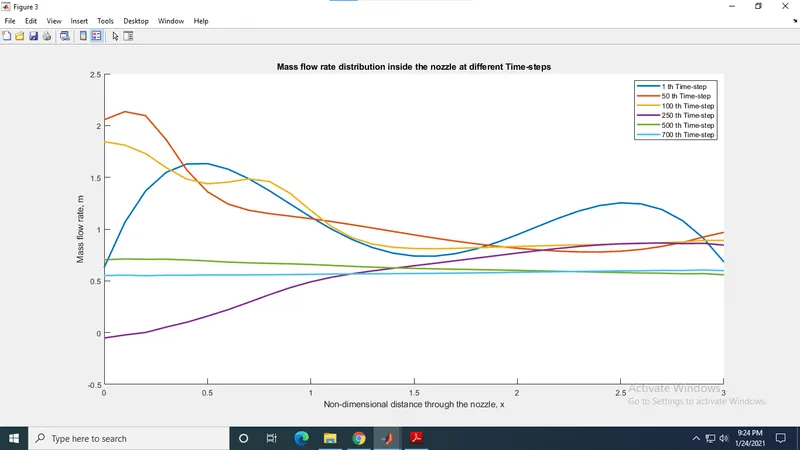
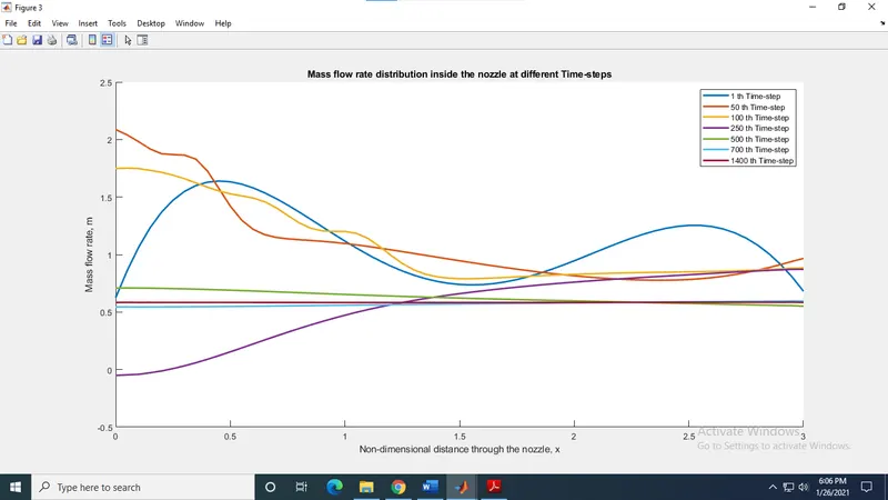
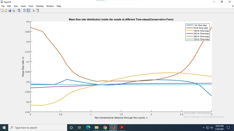
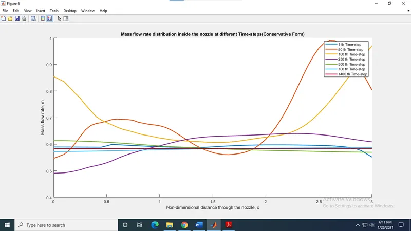
(iii) Mass flow rate distribution inside the nozzle at different time-steps:
Non-Conservation Form (n = 31 & n = 61):
Conservation Form (n = 31 & n = 61):
(iv) Comparison of normalized mass flow rate distribution of both forms:
For n = 31 & n = 61:
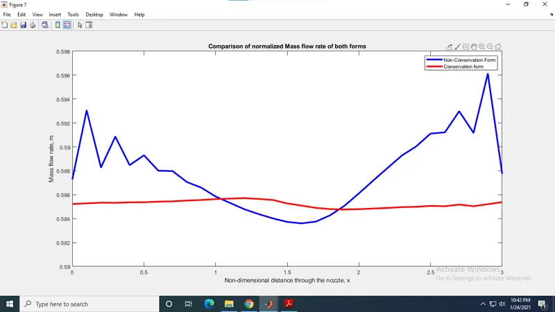
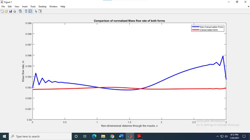
Thus according to the above plots, it is clear that for my criterion of error less than 1%, grid independence has been achieved at 61 grid points when the results from both the forms are compared with the actual analytical results. Still we can increase the number of grid points to 121, but there won't be much variation in the results as we expect it to be. So, in order to save computation time and without compromising the accuracy of the results, I chose 61 grid points to be the better choice for grid independence.
Also the comparison of mass flow rate distribution of both forms shows that the conservation form is more predominant in the results (indicated by an almost horizontal line) than the non-conservation form as the name tells us the conservation form is predominant for mass conservation.
While on a broader picture, it can be concluded that both forms are suitable for solving the quasi 1D nozzle flow problem as both the forms almost represent the same results with minimal error which is obtained by the use of CFL criterion in the solution. The Courant number which was chosen for stability is 0.5 since the conservation part requires too much encoding and decoding due to flux term introduction. But still we must understand that solving using the non-conservative form is much efficient than using conservative form in CFD point of view, although they both produce equally accurate results, the conservative form can produce results of accuracy equal to the non-conservative form but only with twice the number of grid points than used by the non-conservative form.