Week 7 - Simulation of a 1D Super-sonic nozzle flow simulation using Macormack Method

AIM: To simulate the 1D supersonic nozzle flow using Macormack method by deriving both conservative and non conservative forms of the governing differential equations.

THEORY: A study isoentropic flow is considered inside a converging diverging nozzle. The flow at the inlet comes from a reservoir where the velocity is very small and the area is very large. The flow is subsonic at the convergent section, becomes sonic at the throat and supersonic at the diverging section.

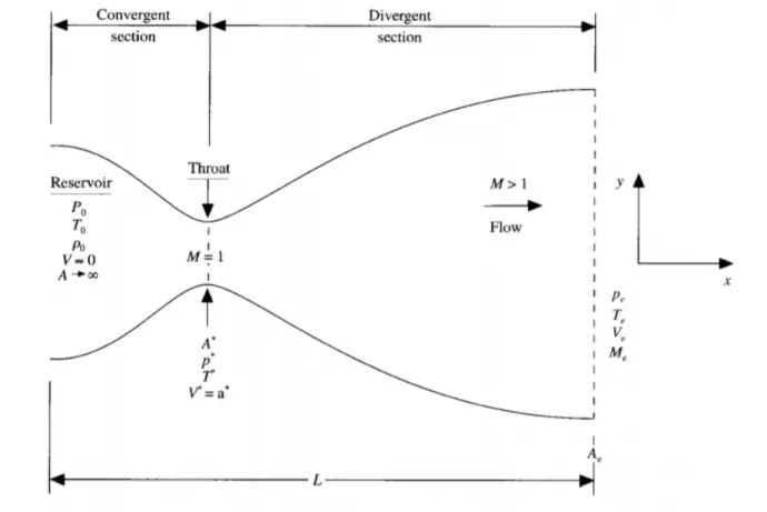
The schematic representation of the nozzle is shown.

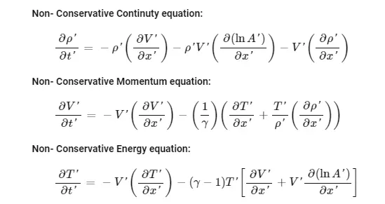
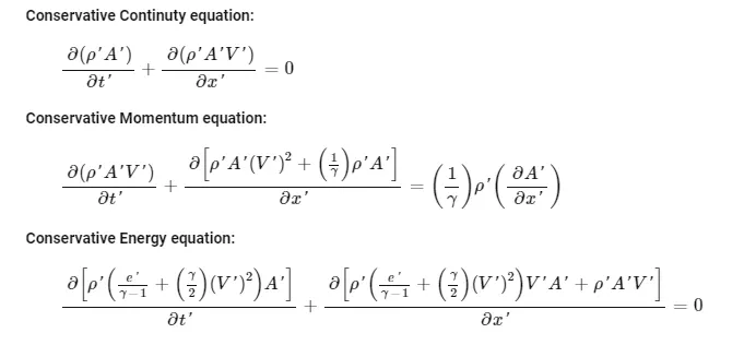
The governing differential equations namely continuity equation, momemtum equation and energy equation are time marched in terms of PDE for both conservative and non conseravative forms.

The non dimensional governing differential equations for non conservative forms are given below:

The non dimensional governing differential equations for conservative forms are given below:

Solving the governing differntial equations using Macormack method:

For the f(x), the following steps are involved:

I) Initial profile definition

The initial profile for all the flow variables have to be defined.

II) Predictor step

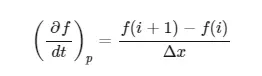
III) Solution update after predictor step:

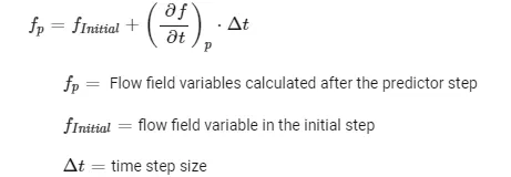
IV) Corrector step:

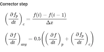
V) Final solution update:

MATLAB CODE FOR calling both conservative and non conservative form functions and plotting:

clear all
close all
clc

n=31; %defining number of grid points
gamma=1.4; 
x=linspace(0,3,n);
dx=x(2)-x(1); % each grid length

nt=1400; %number of time steps
C=0.5; %courant number

%defining functions seperately for non conservative and conservative form
[mf_nc,p_nc,mn_nc,rho_nc,v_nc,t_nc,rho_throat_nc,v_throat_nc,t_throat_nc,mf_throat_nc,p_throat_nc,mn_throat_nc]=nc(x,dx,n,gamma,nt,C);

%Plotting of variation of properties with time
figure(1)
subplot(4,1,1) 
%plotting the density
plot( linspace(1,nt,nt),rho_throat_nc,'color','m')
ylabel('density at the throat');
axis([0 1400 0 1.3]);
grid minor;
title('timestep variation at the throat, Non conservative form')

%plotting the temperature
subplot(4,1,2)
plot( linspace(1,nt,nt),t_throat_nc,'color','c')
ylabel('temperature');
axis([0 1400 0.6 1]);
grid minor;

%plotting pressure
subplot(4,1,3)
plot( linspace(1,nt,nt),p_throat_nc,'color','g')
ylabel('pressure');
axis([0 1400 0.4 1.1]);
grid minor;

%plotting mach number
subplot(4,1,4)
plot( linspace(1,nt,nt),mn_throat_nc,'color','y')
ylabel('mach number');
axis([0 1400 0.6 1.4]);
grid minor;

% now plotting the steady state variables 

figure(3);
subplot(4,1,1)
plot(x,rho_nc,'color','m')
ylabel('density');
axis([0 3 0 1]);
grid minor;
title('steady state flow distribution, non conservative')

subplot(4,1,2)
plot(x,t_nc,'color','c')
ylabel('temperature');
axis([0 3 0 1]);
grid minor;

subplot(4,1,3)
plot(x,p_nc,'color','g')
ylabel('pressure');
axis([0 3 0 1]);
grid minor;

subplot(4,1,4)
plot(x,mn_nc,'color','y')
ylabel('mach number');
axis([0 3 0 4]);
grid minor;

% now defining the function for coservative form

[mf_c,p_c,mn_c,rho_c,v_c,t_c,rho_throat_c,v_throat_c,t_throat_c,mf_throat_c,p_throat_c,mn_throat_c]=c(x,dx,n,gamma,nt,C);

%plotting for conservative form
figure(5)
subplot(4,1,1) 
%plotting the density
plot(rho_throat_c,'color','m')
ylabel('density at the throat');
axis([0 1400 0 1]);
grid minor;
title('timestep variation at the throat,conservative form')

%plotting the temperature
subplot(4,1,2)
plot(t_throat_c,'color','c')
ylabel('temperature');
axis([0 1400 0.6 1]);
grid minor;

%plotting pressure
subplot(4,1,3)
plot(p_throat_c,'color','g')
ylabel('pressure');
axis([0 1400 0.2 0.8]);
grid minor;

%plotting mach number
subplot(4,1,4)
plot(mn_throat_c,'color','y')
ylabel('mach number');
axis([0 1400 0.6 1.4]);
grid minor;

% now plotting the steady state variables 

figure(6);
subplot(4,1,1)
plot(x,rho_c,'color','m')
ylabel('density');
axis([0 3 0 1]);
grid minor;
title('steady state flow distribution,conservative')

subplot(4,1,2)
plot(x,t_c,'color','c')
ylabel('temperature');
axis([0 3 0 1]);
grid minor;

subplot(4,1,3)
plot(x,p_c,'color','g')
ylabel('pressure');
axis([0 3 0 1]);
grid minor;

subplot(4,1,4)
plot(x,mn_c,'color','y')
ylabel('mach number');
axis([0 3 0 4]);
grid minor;

%Comparison of Normalized mass flow rate distributions of both forms

figure(7)
hold on
plot(x,mf_nc,'r','linewidth',1.25)
hold on
plot(x,mf_c,'b','linewidth',1.25)
hold on
grid on
legend(' non conservative','conservative form')
xlabel('length')
ylabel('mass flow rate')

MATLAB code for defining the non conservative form function:

function [mf_nc,p_nc,mn_nc,rho_nc,v_nc,t_nc,rho_throat_nc,v_throat_nc,t_throat_nc,mf_throat_nc,p_throat_nc,mn_throat_nc]=nc(x,dx,n,gamma,nt,C);

%initial boundary conditions
rho_nc=1-0.3146*x;
t_nc=1-0.2342*x;
v_nc=(0.1+1.09*x).*t_nc.^0.5;

%area profile
a=1+2.2*(x-1.5).^2;
throat=find(x==1);

for k=1:nt
    dt=min(C.*dx./(sqrt(t_nc)+v_nc));
    
    rho_old=rho_nc;
    t_old=t_nc;
    v_old=v_nc;
    
    %predictor method
    for j=2:n-1
        % categorizing the different terms of the the equation into simpler
        % variables
        
        dv_dx=(v_nc(j+1)-v_nc(j))/dx;
        drho_dx=(rho_nc(j+1)-rho_nc(j))/dx;
        dt_dx=(t_nc(j+1)-t_nc(j))/dx;
        dlog_a_dx=(log(a(j+1))-log(a(j)))/dx;
        
        %continuity equation
        drho_dt_P(j)=-rho_nc(j)*dv_dx - rho_nc(j)*v_nc(j)*dlog_a_dx-v_nc(j)*drho_dx;
        
        %momemtum equation
        dv_dt_P(j)=-v_nc(j)*dv_dx-(1/gamma)*(dt_dx+(t_nc(j)*drho_dx/rho_nc(j)));
        
        %energy equation
        dt_dt_P(j)=-v_nc(j)*dt_dx-(gamma-1)*t_nc(j)*(dv_dx+v_nc(j)*dlog_a_dx);
        
        %updating the solution after each iteration
        
        rho_nc(j)=rho_nc(j)+drho_dt_P(j)*dt;
        v_nc(j)=v_nc(j)+dv_dt_P(j)*dt;
        t_nc(j)=t_nc(j)+dt_dt_P(j)*dt;
    end
    % corrector method
    for j=2:n-1
        dv_dx=(v_nc(j)-v_nc(j-1))/dx;
        drho_dx=(rho_nc(j)-rho_nc(j-1))/dx;
        dt_dx=(t_nc(j)-t_nc(j-1))/dx;
        dlog_a_dx=(log(a(j))-log(a(j-1)))/dx;
        
        
        %continuity equation
        drho_dt_C(j)=-rho_nc(j)*dv_dx - rho_nc(j)*v_nc(j)*dlog_a_dx-v_nc(j)*drho_dx;
        
        %momemtum equation
        dv_dt_C(j)=-v_nc(j)*dv_dx-(1/gamma)*(dt_dx+(t_nc(j)*drho_dx/rho_nc(j)));
        
        %energy equation
        dt_dt_C(j)=-v_nc(j)*dt_dx-(gamma-1)*t_nc(j)*(dv_dx+v_nc(j)*dlog_a_dx);
        
    end
    
    %computing the average time derivative from predictor and corrector
    %methods
    
    drho_dt=0.5.*(drho_dt_P+drho_dt_C);
    dv_dt=0.5.*(dv_dt_P+dv_dt_C);
    dt_dt=0.5.*(dt_dt_P+dt_dt_C);
    
    %solution update
    
    for i=2:n-1
        rho_nc(i)=rho_old(i)+drho_dt(i)*dt;
        v_nc(i)=v_old(i)+dv_dt(i)*dt;
        t_nc(i)=t_old(i)+dt_dt(i)*dt;
    end
    % boundary conditions
    rho_nc(1)=1;
    v_nc(1)=2*v_nc(2)-v_nc(3);
    t_nc(1)=1;
    
    rho_nc(n)=2*rho_nc(n-1)-rho_nc(n-2);
    v_nc(n)=2*v_nc(n-1)-v_nc(n-2);
    t_nc(n)=2*t_nc(n-1)-t_nc(n-2);
    
    mf_nc=rho_nc.*a.*v_nc;
    p_nc=rho_nc.*t_nc;
    mn_nc=(v_nc./sqrt(t_nc));
    
    % computing variables at throat
    rho_throat_nc(k)=rho_nc(throat);
    t_throat_nc(k)=t_nc(throat);
    v_throat_nc(k)=v_nc(throat);
    mf_throat_nc(k)=mf_nc(throat);
    p_throat_nc(k)=p_nc(throat);
    mn_throat_nc(k)=mn_nc(throat);
    
    %Plotting non dimensional mass flow rates at various timesteps
   
    figure(1)
    if k==100
        plot(x,mf_nc,'m');
        hold on
    elseif k==200
        plot(x,mf_nc,'c');
        hold on
    elseif k==500
        plot(x,mf_nc,'y');
    end
    
    title('mass flow rates at various time steps')
    xlabel('length')
    ylabel('mass flow rate')
    axis([0 3 0 2])
    grid on
end
end

    
    

MATLAB code for defining conservative form function:

function [mf_c,p_c,mn_c,rho_c,v_c,t_c,rho_throat_c,v_throat_c,t_throat_c,mf_throat_c,p_throat_c,mn_throat_c]=c(x,dx,n,gamma,nt,C);
for i=1:n
    if (x(i)>=0 && x(i)<=0.5)
        rho_c(i)=1;
        t_c(i)=1;
    elseif (x(i) >=0.5 &&x(i)<=1.5)
        rho_c(i)=1-0.366*(x(i)-0.5);
        t_c(i)=1-0.167*(x(i)-0.5);
    elseif (x(i)>=1.5 && x(i)<=3)
        rho_c(i)=0.634-0.3897*(x(i)-1.5);
        t_c(i)=0.833-0.3507*(x(i)-1.5);
    end
end

a=1+2.2*(x-1.5).^2;
throat=find(a==1);

v_c=0.59./(rho_c.*a);
p_c=rho_c.*t_c;
%initial soluiton vectors
U1=rho_c.*a;
U2=rho_c.*a.*v_c;
U3=rho_c.*a.*(t_c./(gamma-1))+((gamma/2).*v_c.^2);

for k=1:nt
    dt=min(C.*dx./(sqrt(t_c)+v_c));
    U1_old=U1;
    U2_old=U2;
    U3_old=U3;
    
    %flux vectors
    F1=U2;
    F2=((U2.^2)./U1)+((gamma-1)/gamma)*(U3-(gamma/2)*((U2.^2)./U1));
    F3= ((gamma*U2.*U3)./U1)-(gamma*(gamma-1)*((U2.^3)./(2*U1.^2)));
    
    %calculating the variables through predictor method
    for j=2:n-1
        
        J2(j)=(1/gamma)*rho_c(j)*t_c(j)*((a(j+1)-a(j))/dx);
        
        %continuity equation
        dU1_dt_p(j)=-((F1(j+1)-F1(j))/dx);
        %momemtum
        dU2_dt_p(j)=-((F2(j+1)-F2(j))/dx)+J2(j);
        %energy
        dU3_dt_p(j)=-((F3(j+1)-F3(j))/dx);
        
        %update of values
        U1(j)=U1(j)+dU1_dt_p(j)*dt;
        U2(j)=U2(j)+dU2_dt_p(j)*dt;
        U3(j)=U3(j)+dU3_dt_p(j)*dt;
    end
    F1=U2;
    F2=((U2.^2./U1)+((gamma-1)/gamma)*(U3-((gamma*0.5*(U2.^2))./(U1))));
    F3=((gamma*U2.*U3)./U1)-((gamma+0.5*(gamma-1)*(U2.^3))./(U1.^2));
    
    %calculation of variables through corrector method
    for j=2:n-1
        J2(j)=(1/gamma)*rho_c(j)*t_c(j)*((a(j)-a(j-1))/dx);
        
        dU1_dt_c(j)=-((F1(j)-F1(j-1))/dx);
        dU2_dt_c(j)=-((F2(j)-F2(j-1))/dx)+J2(j);
        dU3_dt_c(j)=-((F3(j)-F3(j-1))/dx);
    end
    
    dU1_dt=0.5*(dU1_dt_p+dU1_dt_c);
    dU2_dt=0.5*(dU2_dt_p+dU2_dt_c);
    dU3_dt=0.5*(dU3_dt_p+dU3_dt_c);
    
    %final solution
    for i=1:n-1
        U1(i)=U1_old(i)+dU1_dt(i)*dt;
        U2(i)=U2_old(i)+dU2_dt(i)*dt;
        U3(i)=U3_old(i)+dU3_dt(i)*dt;
    end
    
    %boundary conditions at the inlet
    U1(1)=rho_c(1)*a(1);
    U2(1)=2*U2(2)-U2(3);
    
    v_c(1)=U2(1)./U1(1);
    U3(1)=U1(1)*((t_c(1)/(gamma-1))+((gamma/2)*(v_c(1)).^2));
    
    %outlet
    u1(n)=2*U1(n-1)-U1(n-2);
    u2(n)=2*U2(n-1)-U2(n-2);
    u3(n)=2*U3(n-1)-U3(n-2);
    
    rho_c=U1./a;
    v_c=U2./U1;
    t_c=(gamma-1)*((U3./U1-(gamma/2)*(v_c).^2));
    
    %defining variables 
    mf_c=rho_c.*a.*v_c;
    p_c=rho_c.*t_c;
    mn_c=(v_c./sqrt(t_c));
    %variables at throat section
    rho_throat_c(k)=rho_c(throat);
    t_throat_c(k)=t_c(throat);
    v_throat_c(k)=v_c(throat);
    mf_throat_c(k)=mf_c(throat);
    p_throat_c(k)=p_c(throat);
    mn_throat_c(k)=mn_c(throat);
    
    %Plotting of variables
    figure(4)
    if k==100
        plot(x,mf_c,'m');
    elseif k==200
        plot(x,mf_c,'c');
    elseif k==400
        plot(x,mf_c,'y');
    end
    
    %labels
    title('mass flow at different time steps-conservative');
    xlabel('length');
    ylabel('mass flow');
    legend({'100th time step','200th time step','400th time step'});
    axis([0 3 0.4 1])
    grid on
end
end

Results and plots:

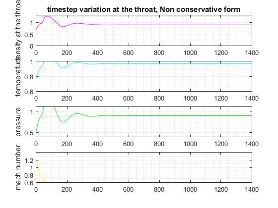
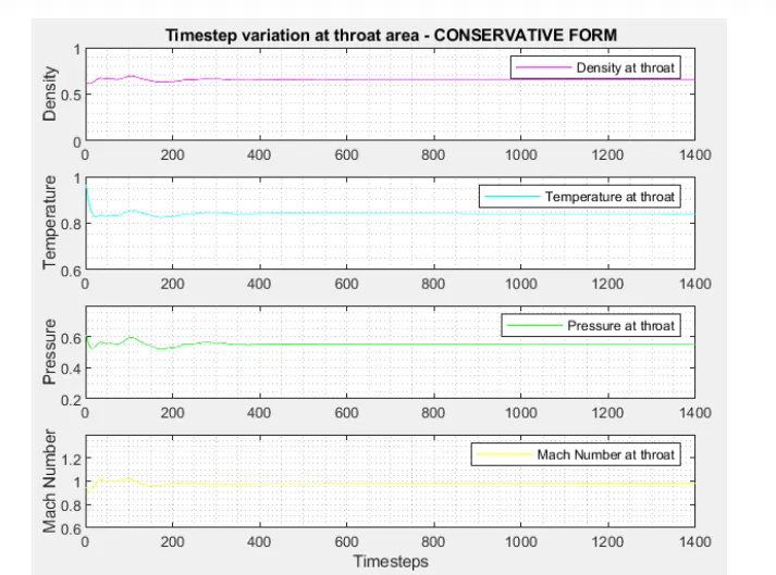
Observe that the time taken to achieve stable solution for non conservative form is higher than that of conservative form.

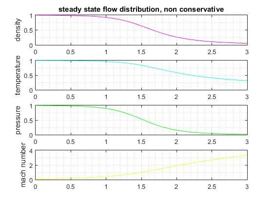
Notice that the plots are almost similar given exactly the same solution.

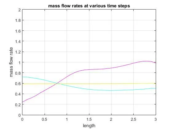
The yellow line represents the 500th time step and hence the solution becomes stable after 500th time step for both the forms.

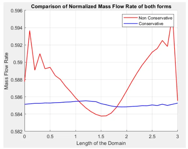
Note that the conservative form attains stability in lesser number of iterations.

GRID INDEPENDENCE TEST:

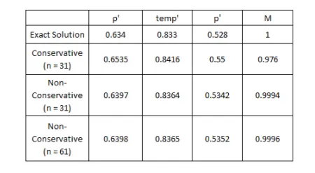
The non conservative form give more accurate results than the conservative form. This occurs because the residuals after each time step are reduced faster in non coservative form.