Week 4 - Genetic Algorithm

AIM: To understand the concept of genetic algorithm and optimise the stalgamite function to find the global maxima.

THEORY: Genetic algorithm reflects the process of natural selection where the fittest individuals are selected for reproduction in ordet to produce offspring for the next generation. The genetic algorithm solves optimization problems by mimicking the principles of biological evolution, repeatedly
modifying a population of individual points using rules modeled on gene combinations in biological reproduction. The advantage is that GA doesnot require the functions to be continuos or differentiable.

GA funcion syntax in MATLAB:

[x,fval]=ga(func, var,A, B,Aeq,Beq,lb,ub,noni,intcon,options)

The output after executing the ga function gives two ouputs if called by two variables.

The 'x' output gives the coordinates of the fucntion minimum and 'fval' is the minimum value of the function.

func= Objective function to be minimised

var =number of variables

A,B = constrainted by linear inequalities of the form Ax<=B

Aeq, Beq =constaints to linear equalities

lb and ub =lower and upper bounds for the inputs respectively.

noni =non linear inequality constraints

intcon= integer constraints

options= adding constraint tolerances by increasing population for more interations

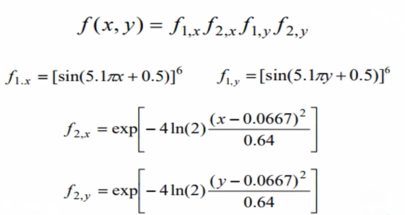
We will be applying genetic algorithm on the stalagmite function. The stalagmite function is given as:

Procedure of GA implementation:

First, the stalagmite function is created using MATLAB. x and y variables are assinged random values and corresponding 2D array is created using meshgrid function. The stalagmite function values are calculated for the meshgrid values and stored in a variable. Then the GA algorithm is implemented for the function values using three different cases to find the maximum function value.The first study case has no bounds to input variables and hence the GA starts by choosing random input values. The second study involves the input variables that are bounded so that the GA searches for the maximum value of the function within the specified bounds for the input variables. The third study include the optimoptions command to consider the population size and improve accuracy.

The code for the stalagmite function is given:

%stalgamite function
function  fv=stalgamite_function(input_vector)
x1=input_vector(1)
y1=input_vector(2)

f1x=[sin(5.1*pi*x1+0.5)]^6;
f1y=[sin(5.1*pi*y1+0.5)]^6;
f2x=exp(-4*log(2)*((x1-0.0667).^2/0.64));

f2y=exp(-4*log(2)*((y1-0.0667).^2/0.64))
fv= -f1x*f1y*f2x*f2y
end

Since the stalgmite function is now defined, we can implement genetic algorithm on the function. The matlab code is given below:

%implementing GA on a stalagmite function

x=linspace(0,0.6,150); %creating a vector for x cooridnates
y=linspace(0,0.6,150); % creating a vector for y coordinates
num_cases=50;  % defining number of loops for running the GA
[xx,yy]=meshgrid(x,y);% creating  a mesh grid of x and y coordinates for plotting surface plots

for i=1:length(xx)  % running through first loop through x coordinates
    for j=1:length(yy) % second loop for running through y coordinates
        input_vector(1)=xx(i,j); % picking x coordinate to input into stalagmite function
        input_vector(2)=yy(i,j); % picking y coordinate to input into stalagmite function
        f(i,j)=stalgamite_function(input_vector); % finding the stalagmite function value for the picked coordiantes
    end
end

tic        
% study 1 - statistical behavior 

%looping through number of cases to run GA algorithm
for i=1:num_cases      
[input,f_val(i)]=ga(@stalgamite_function,2)     % implementing ga algorithm on stalagmite function
i_x(i)=input(1) %extracting the x coordinate result
i_y(i)=input(2) % extracting the y coordiante result
end
study1_time=toc

% plotting the first case figure
figure(1) 
subplot(2,1,1) 
hold on
surfc(xx,yy,f);         %plottin the stalagmite function
xlabel('x value')
ylabel('y value')
hold on
shading interp
plot3(i_x,i_y,f_val,'marker','o','markersize',5)  %plotting the x and y coordinates resulted by GA
title('Unbounded inputs')
subplot(2,1,2)
plot(f_val)    %plotting function value minimum obtained by GA for each iteration.
xlabel('Number of interations')
ylabel('function value minimum')

% study 2, statistical study with lower and upper bounds. Bounded inputs to restrict the input range for GA
tic

for i=1:num_cases
    [input,f_val(i)]=ga(@stalgamite_function,2,[],[],[],[],[0;0],[0.7;0.7])% implemening ga with lower and upper bounds for the x and y coordiantes
    i_x(i)=input(1)
    i_y(i)=input(2)
end
study2_time=toc

% plotting the second case figures
figure(2)
subplot(2,1,1)
hold on
surfc(xx,yy,f);
xlabel('x value')
ylabel('y value')
hold on
shading interp
plot3(i_x,i_y,f_val,'marker','o','markersize',5)
title('Bounded inputs')
subplot(2,1,2)
plot(f_val)
xlabel('Number of interations')
ylabel('function value minimum')

% study 3, Increasing GA interations with bounded inputs to obtain more accurate results.
options= optimoptions('ga');
options= optimoptions(options,'PopulationSize',250)

tic

for i=1:num_cases
    [input,f_val(i)]=ga(@stalgamite_function,2,[],[],[],[],[0;0],[0.7;0.7],[],[],options) %implementing ga with options
    i_x(i)=input(1)
    i_y(i)=input(2)
end
study2_time=toc

%plotting third case figures
figure(3)
subplot(2,1,1)
hold on
surfc(xx,yy,f);
xlabel('x value')
ylabel('y value')
hold on
shading interp
plot3(i_x,i_y,f_val,'marker','o','markersize',5)
title('Bounded inputs with increases GA interations')
subplot(2,1,2)
plot(f_val)
xlabel('Number of interations')
ylabel('function value minimum')

Figures corresponding to study 1:

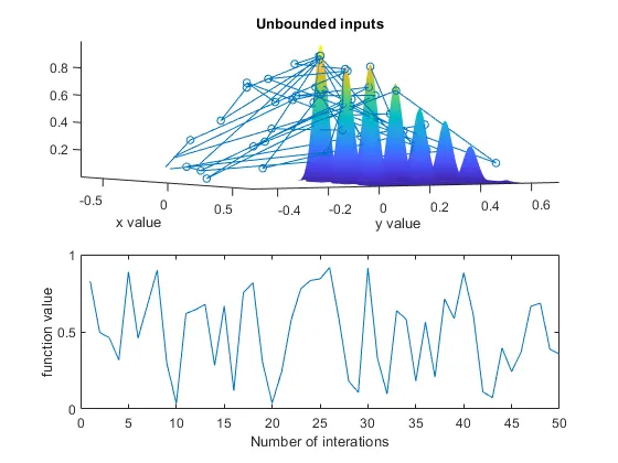
Notice that in the study 1, since there are no bounds to the input values of x and y, the ga tries to find optimum function values by taking random x and y values.

The figures corresponsing to study 2 (bounds to inout variables) are shown:

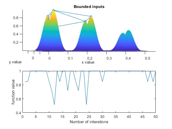
Here since the input variables are bounded, the ga finds the optimum function values by considering only the value for input variables within bounds

Now consider the final study case figures:

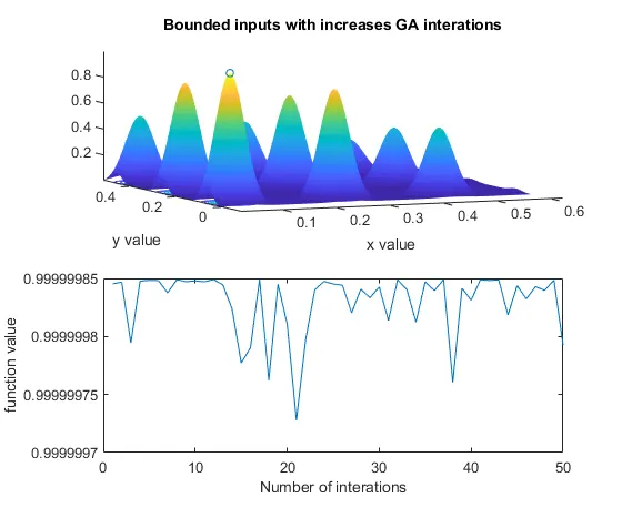
Notice that with a population size of 250, the ga has found a unique maximum value for the function.The coordinates of the function where the maximum and minimum values are attained is x=0.0668 and y=0.0668.

References:

https://in.mathworks.com/help/gads/ga.html

https://www.tutorialspoint.com/genetic_algorithms/genetic_algorithms_introduction.htm