Project 1 - Parsing NASA thermodynamic data

AIM: To write a MATLAB function to extract the 14 coefficients of each species and calculating the specific heat, enthalpy, entropy and molecular weight of each species. To display plots for O2, N2 and CO2 species.

THEORY: The thermodynamic data file by NASA is used to calculate the specific heat, enthalpy and entopies of different species for certain temperature ranges. The formulas to calculate these are given below:

Here Cp, H and S are specific heat, enthalpy and entropy of the species respectively. 'R' is the universal gas constant and 'T' is the temperature at which the property is being calculated.

METHODOLOGY: First,the thermodynamic data is open and read. The header information of global temperature ranges is saved into a variable. Next, using fgetl() command, the lines containing the coefficients are read and the coefficients from each line are recorded and saved into a coefficient vector. After extracting the coefficients, the specific heat, enthalpy, entropy and molecular weights are calculated by calling the respective function which are manually defined. The plots of each species are saved into their respecitve folders. Since there are 53 species, a for loop is used to run the same process for each species.

The MATLAB code for the functions of specific heat, enthalpy, entropy and molecular weights is given below:

%specific heat calculation
function cp=specific_heat(a1,a2,a3,a4,a5,a8,a9,a10,a11,a12,temp,temp_range,R)
for i=1:length(temp_range)
    if temp_range(i)<=temp(2)
        cp(i)=R*(a8+(a9*temp_range(i))+(a10*(temp_range(i).^2))+(a11*(temp_range(i).^3))+(a12*(temp_range(i).^4)));
    else
        cp(i)=R*(a1+(a2*temp_range(i))+(a3*(temp_range(i).^2))+(a4*(temp_range(i).^3))+(a5*(temp_range(i).^4)));
    end
end
end

%enthalpy calculation
function h=enthalpy(a1,a2,a3,a4,a5,a6,a8,a9,a10,a11,a12,a13,temp,temp_range,R)
for i=1:length(temp_range)
    if temp_range(i) <=temp(2)
        h(i)=R*((a8*temp_range(i))+(a9*((temp_range(i).^2)/2))+(a10*((temp_range(i).^3)/3))+(a11*((temp_range(i).^4)/4))+(a12*((temp_range(i).^5)/5))+a13);
    else
        h(i)=R*((a1*temp_range(i))+(a2*((temp_range(i).^2)/2))+(a3*((temp_range(i).^3)/3))+(a4*((temp_range(i).^4)/4))+(a5*((temp_range(i).^5)/5))+a6)
    end
end
end

%entropy calculation function
function s=entropy(a1,a2,a3,a4,a5,a7,a8,a9,a10,a11,a12,a14,temp,temp_range,R)
for i=1:length(temp_range)
    if temp_range(i)<= temp(2)
        s(i)=R*((a8*log(temp_range(i)))+(a9*temp_range(i))+(a10*((temp_range(i).^2)/2))+(a11*((temp_range(i).^3)/3))+(a12*((temp_range(i).^4)/4))+a14)
    else
        s(i)=R*((a1*log(temp_range(i)))+(a2*temp_range(i))+(a3*((temp_range(i).^2)/2))+(a4*((temp_range(i).^3)/3))+(a5*((temp_range(i).^4)/4))+a7)
    end
end
end

        
%molecular weight
function [m_weight]=weight(species_name)
species={'H','O','N','Ar','C','S'};
a_mass=[1.008,16,14,40,12,32]
m_weight=0;
for i=1:length(species_name)
    for j=1:length(species)
        if strcmp(species_name(i),species(j))
            m_weight=m_weight+a_mass(j);
            a=j;
        end
    end
    b=str2num(species_name(i));
    if b>1
        m_weight=m_weight+a_mass(a)*(b-1);
    end
end
end

The MATLAB code for extraction of coefficients and plotting figures of different properties is given below:

%NASA data

f1=fopen('THERMO.dat','r') % reading the .dat file
l1=fgetl(f1); % getting the first line and skipping
l2= fgetl(f1);
global_temp= strsplit(l2,' '); % extracting the temperature values
temp_low= str2num(global_temp{2}); % assinging and coverting the temperature values from char to numbers
temp_med=str2num(global_temp{3});
temp_high=str2num(global_temp{4});
l3=fgetl(f1);
l4=fgetl(f1);
l5=fgetl(f1);
R=8.314 % universal gas constant

for i=1:53 % for loop for running the code for each species
    l_1=fgetl(f1); % getting the first line of the species data
    species_name=l_1(1:5); % extracting the name of the current species
    species_name=deblank(species_name);
    % extracting the local temperature range values and assigning to
    % variables
    local_temp=l_1(49:75);  
    local_temp=strsplit(local_temp,' ');
    localtemp_low=str2num(local_temp{1});
    localtemp_med=str2num(local_temp{3});
    localtemp_high=str2num(local_temp{2});
    localtemp=[localtemp_low localtemp_med localtemp_high];
    
    temp_range=linspace(localtemp_low,localtemp_high,500);
    l_2=fgetl(f1);
    Epos=strfind(l_2,'E'); % getting the position of letter 'E'
    a(1)=str2num(l_2(1:Epos(1)+3)); % extracting the first coefficient for current species and saving it as a vector
    for j=2:5 % for loop to extract coefficients from the second line
        a(j)=str2num(l_2(Epos(j-1)+4:Epos(j)+3));
    end
    l_3=fgetl(f1);
    Epos=strfind(l_3,'E');
    a(6)=str2num(l_3(1:Epos(1)+3));
    for j=7:10 % for loop to extract coefficients from the third line
        a(j)=str2num(l_3(Epos(j-6)+4:Epos(j-5)+3));
    end
    l_4=fgetl(f1);
    Epos=strfind(l_4,'E');
    a(11)=str2num(l_4(1:Epos(1)+3));
    for j=12:14 % for loop to extract coefficients from the fourth line
        a(j)=str2num(l_4(Epos(j-11)+4:Epos(j-10)+3));
    end
    
%specific heat calculation by calling the specific heat function
Cp= specific_heat(a(1),a(2),a(3),a(4),a(5),a(8),a(9),a(10),a(11),a(12),localtemp,temp_range,R)

% Enthalpy calculation
H=enthalpy(a(1),a(2),a(3),a(4),a(5),a(6),a(8),a(9),a(10),a(11),a(12),a(13),localtemp,temp_range,R)

%entropy calculation
S=entropy(a(1),a(2),a(3),a(4),a(5),a(7),a(8),a(9),a(10),a(11),a(12),a(14),localtemp,temp_range,R)
        
%molecular weight calculation
m_weight=weight(species_name);

%saving m_weight
species_w=fopen('species_mass.txt','w');
fprintf(species_w,'Molecular weight of %s is %f',species_name,m_weight);
fclose(species_w);

%Saving each species data in a folder
current_dir=pwd;
mkdir(species_name);
cd(species_name);

%plotting the figures
figure(1)
plot(temp_range,Cp,'linewidth',3);
xlabel('temperature');
ylabel('specific heat');
title(species_name);

figure(2)
plot(temp_range,H,'linewidth',3);
xlabel('temperature');
ylabel('Enthalpy');
title(species_name);

figure(3)
plot(temp_range,S,'linewidth',3);
xlabel('temperature');
ylabel('Entropy');
title(species_name);

%saving images for each species
saveas(1,'specific_heat.jpg');
saveas(2,'enthalpy.jpg')
saveas(3,'entropy.jpg')

cd(current_dir);

%display molecular weight

fprintf('molecular weight of %s=%f',species_name,m_weight)
end

RESULTS:

The molecular weights of the species are displayed in the command window as shown.

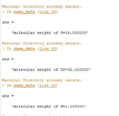
The weights of all the species are shown in the same manner.

The plots of specific heat, enthalpy and entropy for O2, N2 and CO2 species are shown.

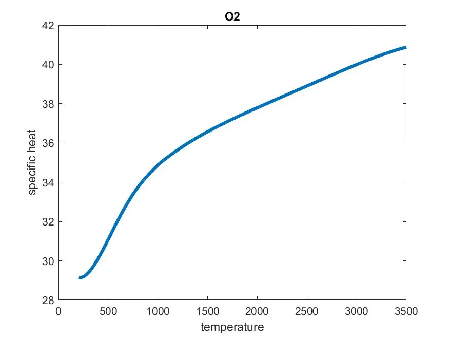
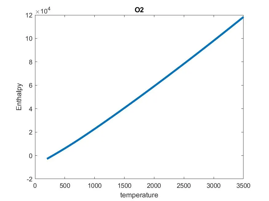
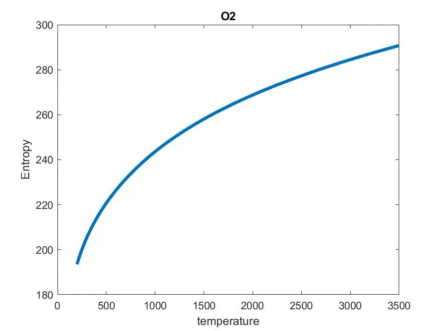
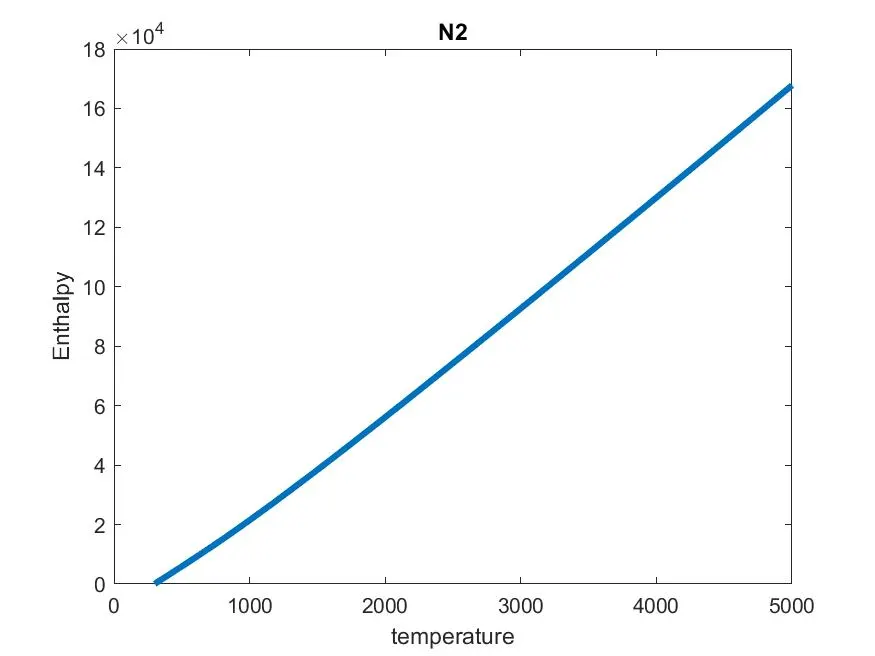
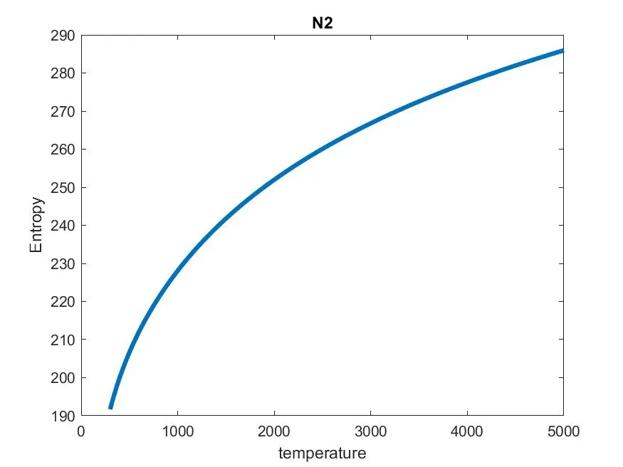
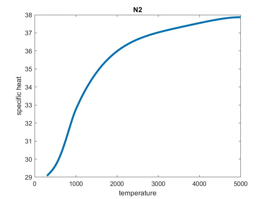
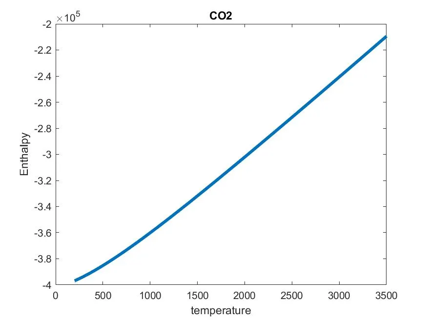
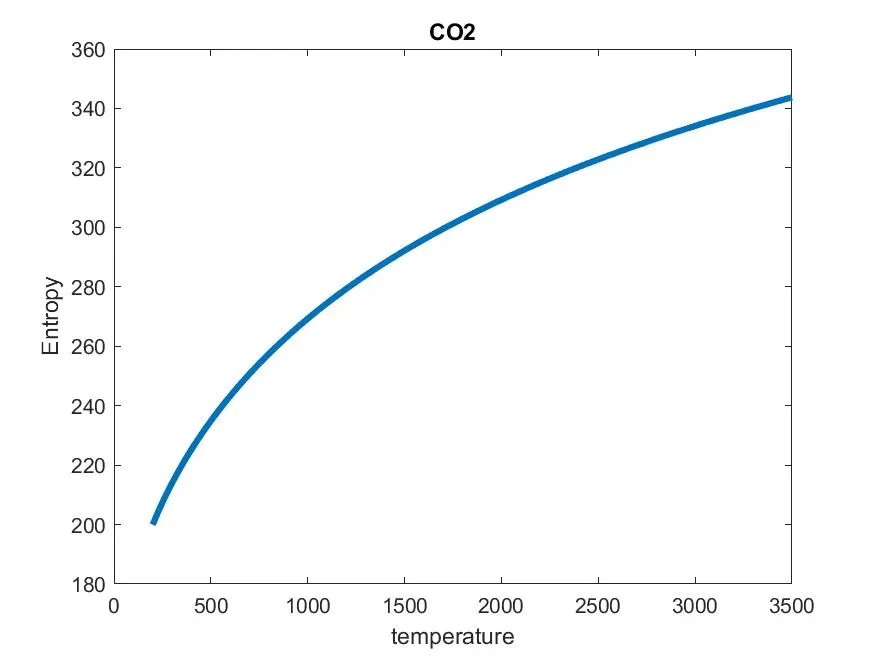
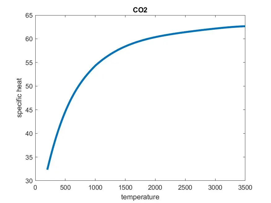Notice that as the temperature increases, the specific heat, enthalpy and entropies increase in different patterns as evident from the plots.

The folders for each species are saved as shown in the figure below:

CONCLUSION:

The thermodnamic coefficients from the NASA's data is extracted and used to find specific heats, enthalpies and entropies for each of the given species and respective curves are plotted. The data for each species is then stored in folders specific to each species.