Week 7 - Simulation of a 1D Super-sonic nozzle flow simulation using Macormack Method
Introduction:
This project deals with the quasi-one-dimensional flow through a convergent divergent nozzle.The isentropic flow through the nozzle is being simulated. The term subsonic-supersonic implies that the flow enters the convergent section of the nozzle ,from the reservoir with mach number less than one and leaves the divergent section of the nozzle with mach number greater than one.Isentropic flow implies that the entropy remains constant and its adiabatic. the working format of the project is first the physical flow will be described including the various governig equations and relationships obtained from the analytical solutionsThen a CFD solution technique will be implemented and finally the results will be plotted through various graphs and tabes.
Theory:
Flow description:
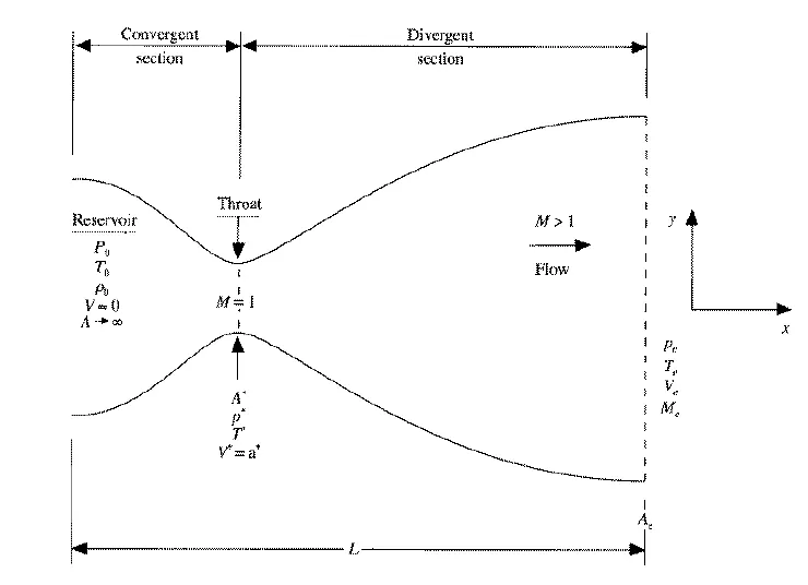 (figure 1)
The above figure is a visualization of a convergent divergent nozzle. The flow at the inlet comes from the reservoir. the area of the reservoir is pretty large and considered to be infinity. So from the continiuty equation , the velocity is very small and is equal to zero. (AV=Constant). . So the pressure and temperature values are the stagnation values. the throat section is the section with minimum cross sectional area.The flow is subsonic in the convergent section , sonic at the throat nd supersonic at the nozzle exit. The stgnation temperature, stagnation pressure ,stagnation density is written as :
`t(0)=t*(1+(gamma-1)/2*M^2)`--(1)
`p(0)=p*(1+(gamma-1)/2*M^2)^(gamma/(gamma-1)`---(2)
`rho(0)=rho*(1+(gamma-1)/2*M^2)^(1/(gamma-1))`----(3)
`M` denotes the mach number .
Mach number can be defined as the ratio of the fluid flow and the speed of the sound in fluid.
For mach number less than or equal to 0.3, the flow is considered to be incompressible and fomach number greater than 0.3 , the flow is compressible.
For perfect gas , the speed of sound is writen as `c = (gamma*R*T)^(1/2)`---(4)
In the throat section the mach number is 1, the properties are called sonic properties and the flow is sonic flow.
the sonic properties are writtenas :
`t(sonic)=2*t(0)*((gamma+1)^-1)`---(5)
`p(sonic)=p(0)*(1+(gamma-1)/2)^((gamma-1)/gamma`---(6)
`rho(sonic)=rho(0)*(1+(gamma-1)/2)^((gamma-1)/gamma`---(7)
The area ratio as a function of mach number in a isentropic nozzle can be represented as :
`a/(a(sonic))=1/M*((2/(gamma-1)*(1+(gamma-1)/2*M^2))^((gamma+1)/(2*(gamma-1))`----(8)
The governing continiuty , momentum,and energy equations for the quasione dimensional steady,isentropic flow can be expressed as :
`rho(1)*a(1)*v(1)=rho(2)*a(2)*v(2)`---(9)
Thisis the continity equation
`p(1)*a(1)+(rho(1)*v(1)^2*a(1))+int_(a(1))^(a(2)) p*da=p(2)*a(2)+(rho(2)*v(2)^2*(a(2))`---(10)
This is the momentum equation
`h(1)+(v(1)^2)/2=h(2)+(v(2)^2)/2`----(11)
This is the energy equation
Since perfect gas is considered;
`p=rho*R*T`---(12)
`dh=c_p*dt`----(13)
`du=c_v*dt`----(14)
`gamma=c_p/c_v`----(15)
With these above equations and relationships the flow can be simulated.
CFD Solution and solution of governing equations:
The governing flow equations are written in partial differential equations that are suitable for time marching solutions of the quasi 1D flow.
The integral form of the continiuty equation is given by :
`del/dt(intintint_v(rho*dV))+intint_S(rhov*dS)=0`---(16)
The `del/(delt)(intintint_V(rho*dV))=del/(delt)(rho*a*dx)`---(17)
teh dx term is the length of the control volume considered for the calculation in the complete nozzle. Adx is the volume of the control volume in the limit dx becoming vanishingly small.
the term `intint_S(rhov*dS)=-rho*v*a+rho*v*da+rho*v*da+rho*a*dv+rho*dv*da+a*v*drho+v*da*drho+a*dv*drho+drho*dv*da`---(18)
the terms involving the differnilas multiplication are ignored as they are way small as dx tends to zero.
subsitituting (17)and (18) in equation (16)
`del/(delt)(rho*A)+del/(delx)(rho*A*v)=0`-----(17)
equation (17) is the partial differential equation form of the continiuty equation , that is applicable for unsteady, quasi one dimensional flow. Since area is constant with respect to x direction and `u`is the x component velocity ,the equation (17) becomes
`(del(rho))/(delt)+(del(rho*u))/(delx)=0`---(18)
Similarly , the momentum equation in integral form can be transformed into partial differential equation form and can be written as (non conservation):
`rho*(delv)/(delt)+rho*v*(delv)/(delx)=-(delp)/(delx)`----(19)
The energy equation can be written as :
`rho*(dele)/(delt)+rho*v*(dele)/(delx)=-p*(delv)/(delx)-p*v*(del(lna))/(delx)`------(20)
Since `p/(p(0)`,`rho/(rho(0)`,`t/(t(0)` are non dimensional and varies between 0 and 1 , plotting them is easier
In the complete project , wherever the term `p,t,rho,v,a`appears , it is the nondimensional form
| `p` | `p/(p(0)` |
| `t` | `t/(t(0)` |
| `rho` | `rho/(rho(0)` |
| `x` | `x/L` |
| `a` | `a/(a(sonic)` |
| `time` | `(time)/(L/(a(0)` |
So replacing the terms with the non dimensional terms in the three non conservative partial differential form of the governing equations and by making adjustments like `gamma=(c_p/c_v)`,`R/c_v=(gamma-1)` the final set of working equations are obtained:
Continiuty equation:
`(delp)/(delT)=-rho*(delv)/(delx)-rho*v*(del(lna))/(delx)-v*(delrho)/(delx)`` ---(21)
Momentum equation
`(delv)/(delT)=-v*(delv)/(delx)-(1/gamma)*((delt)/(delx)+(t/rho)*(delrho)/(delx))`---(22)
Energy equation:
`(delt)/(delT)=-v*(delt)/(delx)-(gamma-1)*t*((delv)/(delx)+v**(del(lna))/(delx))`---(23)
Matlab coding for the non conservative part:
To solve the above derived partial differential equations , finite difference equations are set up . maccormack technique is followed to solve. Maccormack technique is used for explicit schemes. It uses apredictor corrector philosophy to solve the set of equations.
Since the flow problem considered is One dimensional , the x-axis is divided into finite grid points. `deltax`is the grid spacing.
since it is a timr marching approach , values are solved time point `T+deltaT`from the known values at time point `T`
- Initial profiles of area, density,temperature and velocity are described in form of a equation inside the function for non conservative form.Since it is a convergent divergent nozzle , the profile must look like that
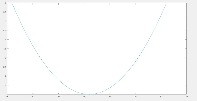 figure(2)
The above is the area profile .
- mass flow rate (m), Mach number(M),pressure ratio or the non dimensional pressure is defined . Care is taken for the dot product, since scalar values. CFL value is 0.5.
- Number of time steps is 1400. inside the time loop , with k being the loop counter variable , the primitive values are first updated . Forthe predictor step , the loop starts from the second node and ends to the second last node. Boundary conditions are provided to the first and the last node. j is the loop counter variable and the for loop is j=2:n-1.
- The complete partial differential equations are broken down into small meaningful parts . Forward difference sceme is used in predictor method.the solution is updated after the predictor step.
- In the corrector step, backward differemncing scheme is used .
- The average time derivative is calculated by averaging the predicted and the corrected values .
- In the final solution update , within a for loop with i as the loop counter variable and the loop starts from node 2 to the (n-1)th loop , the , density,velocity and temperature values are obtained by adding the time derivative obtained by averaging and adding the old values stored
- Boundary conditions are provided as
`v(1)=2*v(2)-v(3)` This is the inlet boundary condition . For the subsonic flow at the inlet
`v(n)=2*v(n-1)-v(n-2)`
`rho(n)=2*rho(n-1)-rho(n-2)`
`t(n)=2*t(n-1)-t(n-2)`
The above sets of equation are the exit boundary conditions for the temperature,velocity and density.
- The values of the variables like mass flow rate, Mach number , density , temperature are found out at throat section and stored as an array .
The matlab code for the non conservation form function is provided below.
function[v,t,rho,m,M,p,t_th,rho_th,M_th,p_th,m_th]= non_con(x,dx,n,a,gamma,nt)

C=0.5;%CFL
%initial profiles
rho = 1-0.3146*x;%density
t = 1-0.2314*x;%temerature
v = (0.1+1.09*x).*t.^0.5;%velocity

dt = min(C*(dx./((t.^0.5)+v)));%time steps
throat = find(a==1);


%defining properties
%mach number
M = v./(t.^0.5);
%pressure ratio
p=rho.*t;
%mass flow rate
m = rho.*a.*v;


%outer time loop
for k =1:nt

    rho_old = rho;
    v_old = v;
    t_old = t;
    %predictor method
    for j = 2:n-1
        dvdx=(v(j+1)-v(j))/dx;
        drhodx=(rho(j+1)-rho(j))/dx;
        dtdx=(t(j+1)-t(j))/dx;
        dlogadx=(log(a(j+1))-log(a(j)))/dx;

        drhodt_p(j) = -rho(j)*dvdx-rho(j)*v(j)*dlogadx-v(j)*drhodx;
        dvdt_p(j) = -v(j)*dvdx-(1/gamma)*(dtdx+(t(j)/rho(j))*drhodx);
        dtdt_p(j) = -v(j)*dtdx-(gamma-1)*t(j)*(dvdx+v(j)*dlogadx);
        %solution update
        rho(j)=rho(j)+drhodt_p(j)*dt;
        v(j)=v(j)+dvdt_p(j)*dt;
        t(j) = t(j)+dtdt_p(j)*dt;
    end
    %corrector step
     for j = 2:n-1

        dvdx=(v(j)-v(j-1))/dx;
        drhodx=(rho(j)-rho(j-1))/dx;
        dtdx=(t(j)-t(j-1))/dx;
        dlogadx=(log(a(j))-log(a(j-1)))/dx;

        drhodt_c(j) = -rho(j)*dvdx-rho(j)*v(j)*dlogadx-v(j)*drhodx;
        dvdt_c(j) = -v(j)*dvdx-(1/gamma)*(dtdx+(t(j)/rho(j))*drhodx);
        dtdt_c(j) = -v(j)*dtdx-(gamma-1)*t(j)*(dvdx+v(j)*dlogadx);
     end
     %compute the average time derivtive
     drhodt = 0.5*(drhodt_p+drhodt_c);
     dvdt = 0.5*(dvdt_p+dvdt_c);
     dtdt = 0.5*(dtdt_p+dtdt_c);

     %final solution update
     for i = 2:n-1
         rho(i)=rho_old(i)+drhodt(i)*dt;
         v(i)=v_old(i)+dvdt(i)*dt;
         t(i)=t_old(i)+dtdt(i)*dt;
     end
     %apply boundary conditions
     %inlet
     v(1)=2*v(2)-v(3);
     %OUTLET
     v(n)=2*v(n-1)-v(n-2);
     rho(n)=2*rho(n-1)-rho(n-2);
     t(n) = 2*t(n-1)-t(n-2);

     m = rho.*a.*v;
     p = rho.*t;
     M = v./t.^0.5;

     %initialising the proprirs value at the throat section
     rho_th(k)=rho(throat);
     v_th(k)=v(throat);
     t_th(k)=t(throat);
     p_th(k)=p(throat);
     M_th(k)=M(throat);
     m_th(k)=m(throat);
    %plotting mass flow rates at different time steps
     figure(1)
     hold on
     if k ==100
         plot(x,m,'linewidth',1.5)
         hold on
     elseif k == 200
         plot(x,m,'linewidth',1.5)
         hold on
     elseif k ==300
         plot(x,m,'linewidth',1.5)
         hold on
     elseif k==500
         plot(x,m,'linewidth',1.5)
         hold on
     elseif k == 700
         plot(x,m,'linewidth',1.5)
         hold on
     elseif k ==1400
         plot(x,m,'linewidth',1.5)
         hold on
     end

xlabel('distance in nozzle')
ylabel('mass flow rate')
legend('100 time steps','200 time steps','300 time steps','500 time steps','700 time steps','1400 time steps')
grid on
grid minor
end
end
Conservative form:
The partial differential equations in the conservative form for the continiuty, momentum and energy equations are as fiollows :
`(del(rho*a))/(delT)+(del(rho*a*v))/(delx)=0`----(24)
This is the continiuty equation
`(del(rho*a*v))/(delT)+(del(rho*a*v^2+(1/gamma)*p*a)/(delx))=(1/gamma)*p*(dela)/(delx)`-----(25)
this is the momentum equation
Defining a non dimensional internal energy , `e=e/(e(0)` and `e(0)=R*(t(0))/(gamma-1)`
`del((rho*(e/(gamma-1))+(gamma/2)*v^2)*a)/(delT)+del(rho*(e/(gamma-1))+(gamma/2)*v^2)*a*v+rho*a*v)/(delx)=0`---(26)
this is the energy equation
By defining elements of the solution vector as U, flux vectors as F and source term as J;
`U1=rho*a`---(27)
`U2=rho*a*v`---(28)
`U3=rho*(e/(gamma-1)+(gamma/2)*v^2)*a`---(29)
`F1=rho*a*v`----(30)
`F2=rho*a*v^2+(1/gamma)*rho*a`----(31)
`F3=rho*(e/(gamma-1)+(gamma/2)*v^2)*v*a+rho*a*v`---(32)
`J2=1/gamma*rho*(dela)/(delx)`------(33)
using these equations from (27) to (33) , the equations from (24) to (26) can be written as:
`(delU1)/(delT)=-(delF1)/(delx)`---(34)
`(delU2)/(delT)=(delF2)/(delx)+J2`----(35)
`(delU3)/(delT)=(delF3)/(delx)`-----(36)
Decoding the terms :
`rho=(U1)/a`---(37)
`v=(U2)/(U1)`---(38)
`t=(gamma-1)*((U3)/(U1)-(gamma/2)*v^2)`----(39)
`p=rho*t`----(40)
from equation(37) to (40) these are the primitive variables.
Matlab coding for the conservative part:
- Everything is as the non conservative part except the predictor, corrector step. The boundary conditons is as as follows:
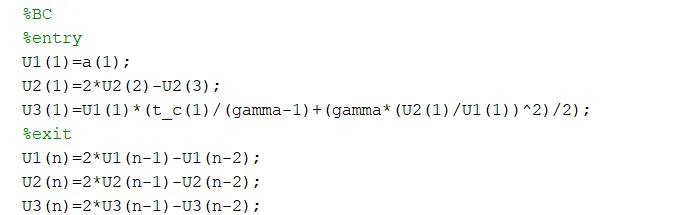 figure(3)
- The initial condition is written in a if loop as:
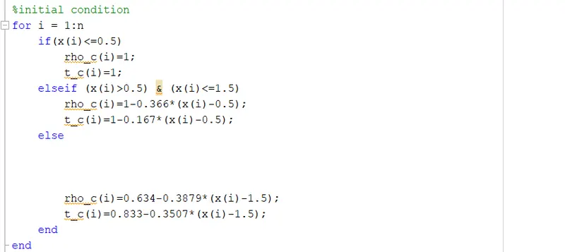 figure(4)
The matlab code for the conservative function is below:
function[v_c,t_c,rho_c,m_c,M_c,p_c,t_thc,rho_thc,M_thc,p_thc,m_thc]= conservative_function(x,dx,n,a,gamma,nt)

%initial condition
for i = 1:n
    if(x(i)<=0.5)
        rho_c(i)=1;
        t_c(i)=1;
    elseif (x(i)>0.5) & (x(i)<=1.5)
        rho_c(i)=1-0.366*(x(i)-0.5);
        t_c(i)=1-0.167*(x(i)-0.5);
    else


        rho_c(i)=0.634-0.3879*(x(i)-1.5);
        t_c(i)=0.833-0.3507*(x(i)-1.5);
    end
end
%solution vector
U1=rho_c.*a;
U2=0.59*ones(1,n);
v_c=U2./U1;
U3=((t_c./(gamma-1))+(gamma*0.5.*(v_c.^2))).*U1;
p_c=rho_c.*t_c;

C=0.5;%CFL

dt = min(C*(dx./((t_c.^0.5)+v_c)));%time step calculation

m_c = rho_c.*a.*v_c;%mass flow rate
throat=find(a==1);
M_c=v_c./(t_c.^0.5);%mach number

%time loop
for k=1:nt
    %storing initial values
    U1_old=U1;
    U2_old=U2;
    U3_old=U3;

    %space loop
    for j =2:n-1
        %flux terms

        F1=U2;
        F2=((U2.^2)./U1)+((gamma-1)/gamma)*(U3-((gamma/2)*(U2.^2))./U1);
        F3=((gamma.*U2.*U3)./U1)-((gamma*(gamma-1)/2)*(U2.^3)./(U1.^2));
        %source term
        J1=(1/gamma)*rho_c(j)*t_c(j)*((a(j+1)-a(j))/dx);
        %predictor step
        du1_dt_p(j)=-(F1(j+1)-F1(j))/dx;
        du2_dt_p(j)=-(F2(j+1)-F2(j))/dx+J1;
        du3_dt_p(j)=-(F3(j+1)-F3(j))/dx;

        %updating solution vector
        U1(j)=U1_old(j)+du1_dt_p(j)*dt;
        U2(j)=U2_old(j)+du2_dt_p(j)*dt;
        U3(j)=U3_old(j)+du3_dt_p(j)*dt;
        %updating primitive values
        rho_c=U1./a;
        t_c=(gamma-1).*(U3./U1-(gamma/2).*(U2./U1).^2);
        %updating flux terms
        F1=U2;
        F2=U2.^2./U1+((gamma-1)/gamma).*(U3-(gamma/2)*U2.^2./U1);
        F3=gamma.*U2.*U3./U1-0.5*gamma*(gamma-1).*U2.^3./U1.^2;
        %source term for c0rrector step
        J2=(1/gamma)*(rho_c(j)*t_c(j)*(a(j)-a(j-1))/dx);
        %corrector step
        du1_dt_c(j)=-(F1(j)-F1(j-1))/dx;
        du2_dt_c(j)=-(F2(j)-F2(j-1))/dx+J2;
        du3_dt_c(j)=-(F3(j)-F3(j-1))/dx;
    end

    du1_dt_avr=0.5*(du1_dt_p +du1_dt_c);
    du2_dt_avr=0.5*(du2_dt_p + du2_dt_c);
    du3_dt_avr=0.5*(du3_dt_p + du3_dt_c);

    for h=2:n-1
        U1(h)=U1_old(h)+du1_dt_avr(h)*dt;
        U2(h)=U2_old(h)+du2_dt_avr(h)*dt;
        U3(h)=U3_old(h)+du3_dt_avr(h)*dt;
    end
    %BC
    %entry
    U1(1)=a(1);
    U2(1)=2*U2(2)-U2(3);
    U3(1)=U1(1)*(t_c(1)/(gamma-1)+(gamma*(U2(1)/U1(1))^2)/2);
    %exit
    U1(n)=2*U1(n-1)-U1(n-2);
    U2(n)=2*U2(n-1)-U2(n-2);
    U3(n)=2*U3(n-1)-U3(n-2);
    %final update
    rho_c=U1./a;
    v_c=U2./U1;
    t_c=(gamma-1).*(U3./U1-(gamma/2).*(U2./U1).^2);
    p_c=rho_c.*t_c;
    M_c=v_c./t_c.^0.5;
    m_c=rho_c.*a.*v_c;
    %throat values
    t_thc(k)=t_c(throat);
    M_thc(k)=M_c(throat);
    m_thc(k)=m_c(throat);
    p_thc(k)=p_c(throat);
    v_thc(k)=v_c(throat);
    rho_thc(k)=rho_c(throat);
    %plotting mass flow rates at different time steps
    figure(5)
    if k==50
        plot(x,m_c,'linewidth',1.5)
        hold on
        grid on

    elseif k==100
        plot(x,m_c,'linewidth',1.5)
        hold on
        grid on

    elseif k ==200
        plot(x,m_c,'linewidth',1.5)
        hold on
        grid on


    elseif k==300
        plot(x,m_c,'linewidth',1.5)
        hold on
        grid on


    elseif k==500
        plot(x,m_c,'linewidth',1.5)
        hold on
        grid on


    elseif k==700
        plot(x,m_c,'linewidth',1.5)
        hold on
        grid on


    elseif k==1400
        plot(x,m_c,'linewidth',1.5)
        hold on
        grid on


    end


end
figure(5)
legend('50 time steps','100 time steps','200 time steps','500 time steps','700 time steps','1400 time steps')
xlabel('Nozzle length')
ylabel('Mass flow rates at different time steps')
grid on
grid minor


end
In the main script , the two functions are called , the conservative and the non conservative. different plots are plotted like the Mach number with respect to nozzle length, temperature with respect to nozzle length,density with respect to nozzle length etc , for both conservative and non conservative form
The matlab code is as follows:
%main script
close all
clc
%inputs
n = 31;                                               %no of grid points
x = linspace(0,3,n);                                  %1dimensional
dx=x(2)-x(1);                                         %grid spacing
a = 1+(2.2*(x-1.5).^2);                               %area
gamma= 1.4;                                           %c_p/c_v
nt = 1400;                                            %no of time steps
%to evaluate time needed for simulation
tic                                                   %starting the timer
%calling the non conservative form equation
[v,t,rho,m,M,p,t_th,rho_th,M_th,p_th,m_th]=non_con(x,dx,n,a,gamma,nt);
simulation_time_nonconseravtive_form =toc
%calling the conservative form
tic%starting the timer
[v_c,t_c,rho_c,m_c,M_c,p_c,t_thc,rho_thc,M_thc,p_thc,m_thc]= conservative_function(x,dx,n,a,gamma,nt);
simulation_time_conservative = toc

%plotting the various steady state variables
figure(2)%new figure window
title('steady state distribution of the propertes')
%Temperature
subplot(4,1,1)
plot(x,t,'linewidth',1.5)

xlabel('Length of nozzle')
ylabel('Non dimensional temperature distribution')
grid on
grid minor
hold on
%Mach number
subplot(4,1,2)
plot(x,M,'linewidth',1.5)
grid on
xlabel('Length of nozzle')
ylabel('Mach number')
hold on
%Density
subplot(4,1,3)
plot(x,rho,'linewidth',1.5)
xlabel('Length of nozzle')
ylabel('Non dimensional density variation')
grid on
hold on
%Pressure variation
subplot(4,1,4)
plot(x,p,'linewidth',1.5)
xlabel('Length of nozzle')
ylabel('Non dimensional pressure variation')
grid on
hold on

%plotting hte variation of parameters with resprct to time at the throat
%section
%T denotes time
T = 1:nt;
figure(3)
%Mach number at throat
subplot(4,1,1)
plot(T,M_th,'linewidth',1.5)

xlabel('time steps')
ylabel('M_Throat')

grid on
hold on
%Density at throat
subplot(4,1,2)
plot(T,rho_th,'linewidth',1.5)

xlabel('Time steps')
ylabel('RHO_Throat')

grid on
hold on
%Temperature at throat
subplot(4,1,3)
plot(T,t_th,'linewidth',1.5)

xlabel('Time steps')
ylabel('T_throat')
grid on
hold on
%pressure variation at throat
subplot(4,1,4)
plot(T,p_th,'linewidth',1.5)

xlabel('time steps')
ylabel('p_Throat')

grid on
hold on

%for the conservative form
figure(4)
title('steady state variables plot')
subplot(4,1,1)
grid on
grid minor
plot(x,M_c,'linewidth',1.5)
xlabel('Nozzle length')
ylabel('Mach number')

subplot(4,1,2)
grid on
grid minor
plot(x,rho_c,'linewidth',1.5)
xlabel('Nozzle length')
ylabel('Non dimensional density')

subplot(4,1,3)
grid on
grid minor
plot(x,p_c,'linewidth',1.5)
xlabel('Nozzle length')
ylabel('Non dimensional pressure')

subplot(4,1,4)
grid on
grid minor
plot(x,t_c,'linewidth',1.5)
xlabel('Nozzle length')
ylabel('Non dimensional temperature')

T=1:nt;
figure(6)
subplot(4,1,1)
plot(T,M_thc,'linewidth',1.5)
grid on
grid minor
ylabel(M_thc)
subplot(4,1,2)
plot(T,rho_thc,'linewidth',1.5)
grid on
grid minor
ylabel('rho_thc')
subplot(4,1,3)
plot(T,p_thc,'linewidth',1.5)
grid on
grid minor
ylabel('p_thc')
subplot(4,1,4)
plot(T,t_thc,'linewidth',1.5)
ylabel('t_thc')
grid on
grid minor
%plotting the mass flow rates at steady state for both the forms
figure(7)
plot(x,m_c,'linewidth',1.5)
hold on
plot(x,m,'linewidth',1.5)
hold on
xlabel('nozzle length')
ylabel('mass flow rate for non conservative and conservative flow')
legend('conservative form','non conservative form')
grid on
grid minor
OUTPUT:
- Plotting mass flow rates with resoect to different time steps for non conservative form:
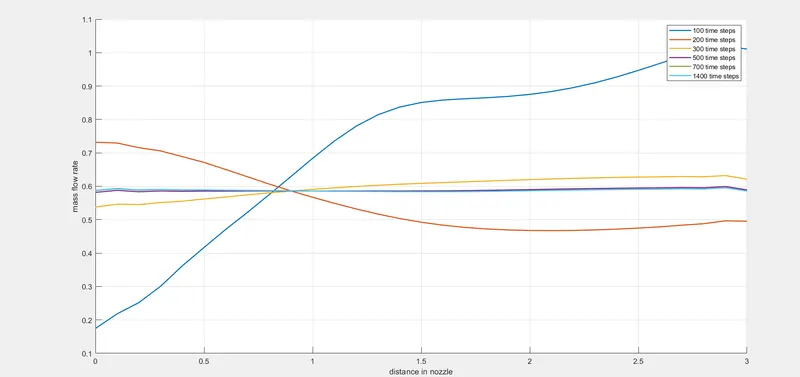 figure(5)
At different time steps, using if and elseif command , the mass flow rates are plotted against the distance in the nozzle that is non dimensional length.
From the plot it can be inferred that at around 500 time steps and more , the curves are more or less straight line.
- Plotting the mass flow rate with respect to nozzle distance at different time steps for the conservative form:
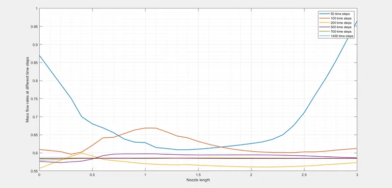 figure(6)
From the plot it can be inferred that the mass flow rates curve get flatter at around 500 time steps and above.
- Plot of the steady state primitive variable distribution within the nozzle for the non conservative form:
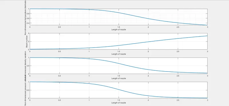 figure(7)
As the length of the nozzle is plotted along the x axis and the various primitive variables along the y axis, The Mach number varies from 0 at the inlet to a value beyond 1, at the supersonic flow at outlet.
- Plot of the steady state primitive variable distribution within the nozzle for the conservative form:
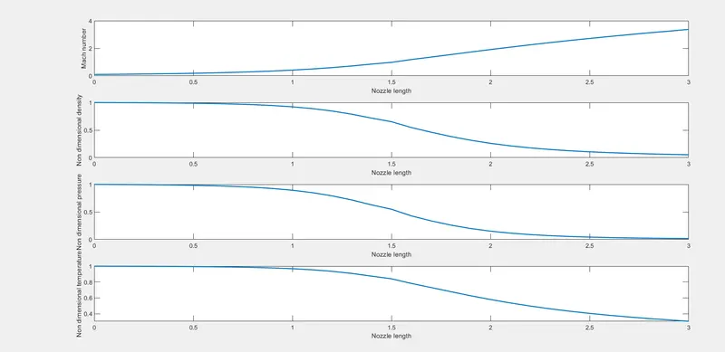 figure(8)
It can be inferred that there is no stark difference between the plots obtained from conservative and non conservative form.
- time wise variation of primitive variables in the throat section of non conservative form:
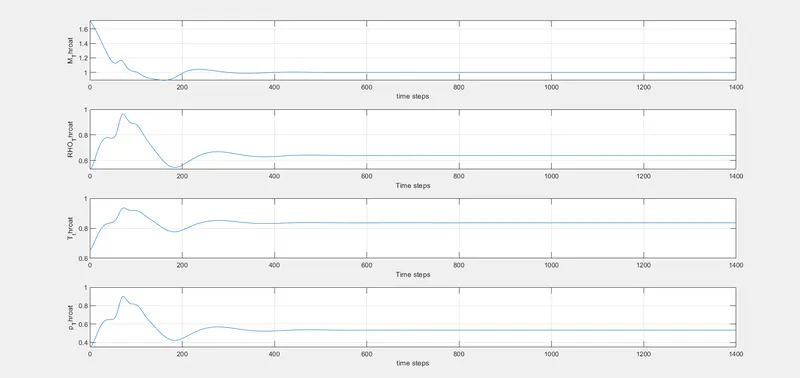 figure(9)
Here it can be seen that initially there are changes at the initial stage , but as the time step increases the primitive variables reaches steady state. At throat the Mach number is 1, after nearly 400 time steps , the the Mach number reaches steady state. same is for all other primitive variables. this is called rubber band effect. Initially the rubber band is stretched tightly and the flow field variables are driven by larger potential so the change is more. after few time steps, it dies down and the steady state is reached.
- Time wise variation of primitive variables in the throat section of conservative form:
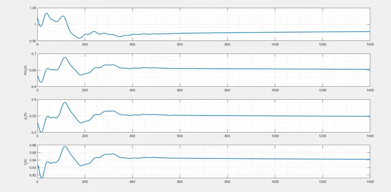 figure(10)
- Plot of the normalized mass flow rates for conservative and non conservative form:
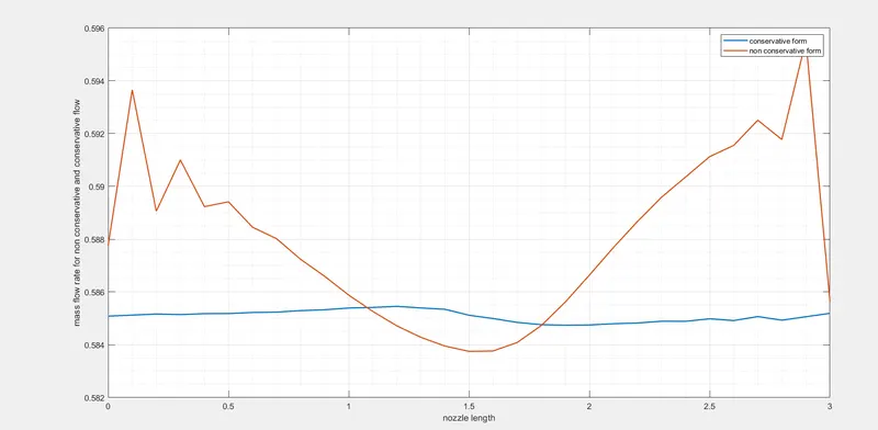 figure(11)
From the above plot it can be inferred that the , normalised mass flow rate in the non conservative form shows more fluctuation with respect to conservative form , in the same flow problem.
- Simulation time:
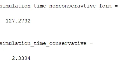 figure(11)
The non conservative form took more time to complete simulation.
Conclusion:
The flow module is completely described, the governing equations derived and the CFD solution is set up. A technique called Maccormack method is utilised. The plots obtained when compared with the analytical results shows similar results