Week 7: Shock tube simulation project

Aim: - To setup a transient Shock-Tube simulation.

Objective: -

1. To setup a transient Shock Tube simulation with N₂ and O₂ as high- and low-pressure zone respectively.
2. To plot the pressure and temperature history for entire domain.
3. To show the change in N₂ mass fraction along with velocity with respect to time.

Theory: -

Shock Tube –

Shock tubes are devices for studying the flow of high-temperature and high-velocity compressible gas. A high-temperature supersonic gas flow is initiated in a shock tube as a result of rupture of a diaphragm or by mechanical driven plunger or by explosive charge, separating two gases in high-pressure and low-pressure chambers.

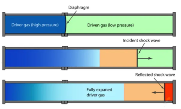
Low pressure gas region is called "driven", which is subjected to the shock wave. High pressure gas region is known as a "driver".

Geometric Model –

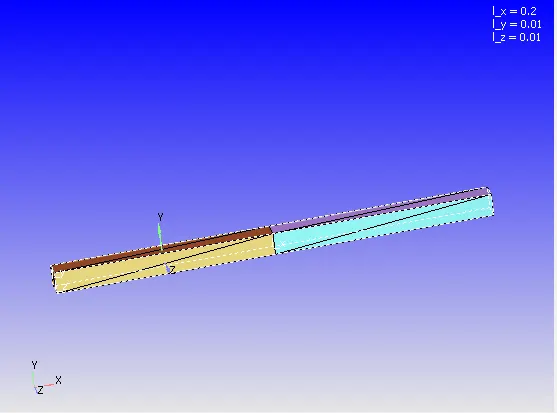
The rectangular tube is divided into 2 halves on containing High Pressure gas and other at Low Pressure. The cross-section area is 1 cm*1 cm and length is 20 cm.

Case Setup –

1. Time Based application type.
2. Gas simulation with Air as predefined mixture.

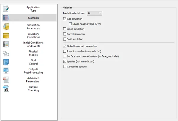
3. Species N2 and O2 are added to the species list.
4. Density Based Transient State Solver is used with Compressible Gas Flow solver and PISO Navier-Stokes’s solver scheme.
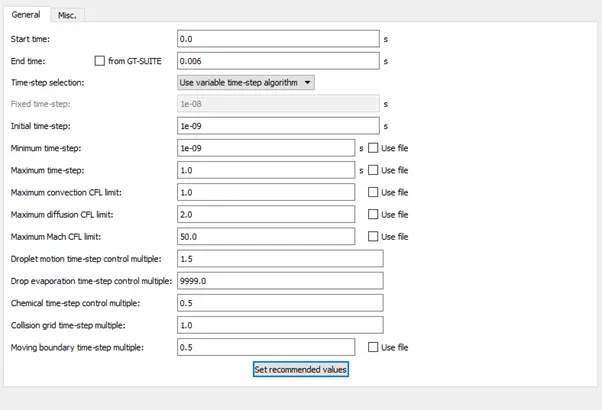
5. The solution run for 0.006 sec with minimum time step of 1e-9 sec and maximum up to 1 sec.

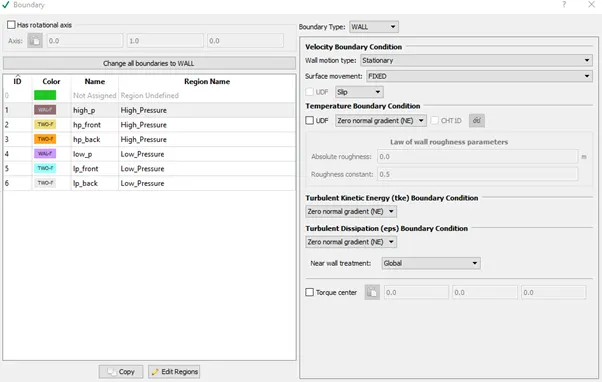
6. Boundary Condition:
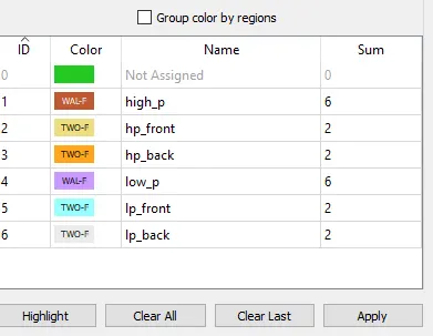
   1. high_p – Type = wall, slip Condition, Region – High_Pressure
   2. low_p – Type = wall, slip Condition, Region – Low_Pressure
   3. Rest all are 2-D Boundaries.

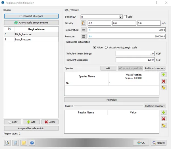
6. High_Pressure Region is initialized with Temperature 300, Pressure 600000 Pa and mass fraction of N2: 1.

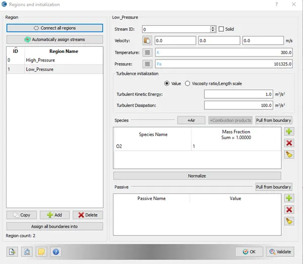
8. Low_Pressure Region is initialized with Temperature 300, Pressure 101325 Pa and mass fraction of O2: 1

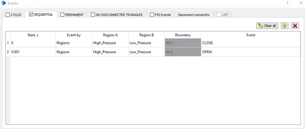
9. Event is marked in initial condition and events tab to specify rupture of diaphragm.

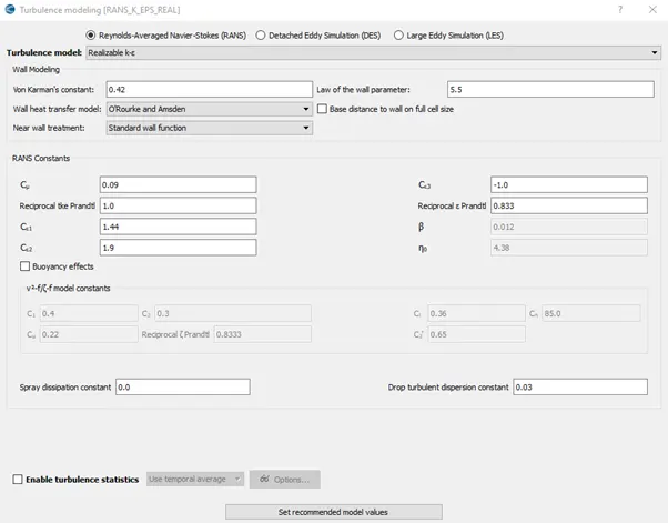
10. Realizable K-epsilon is used for turbulence modelling with recommended values.

11. Base grids of 0.001 m or other for respective cases are generated for all axis.
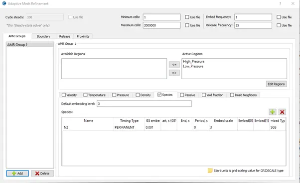
12. Adaptive Mesh Refinement is marked in grid control tab.
13. 
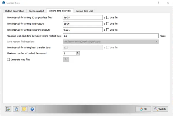
14. Mass Fraction and Species Density for N2 and O2 is checked in post variable output. 3D output data is written after every 5e-5 sec.

14. The input files are exported to a folder to further solving.

Solving using Cygwin:

The Cygwin directory is navigated to the above saved folder and following code is entered to solve the problem.

mpiexec.exe -n 2 "C:\Program Files\Convergent_Science\CONVERGE\3.0.16\bin\intelmpi\converge.exe" restricted </dev/null> logfile &

where address in quotes gives the path of folder containing input file exported earlier.

Post-Processing:

Post-Processing is done with the help of Converge CFD post processing tab –

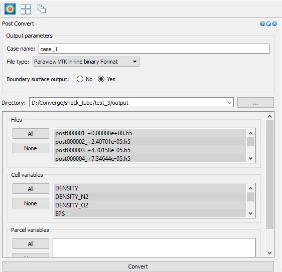
with these the output 3D data is converted in ‘. vtm’ file and contours and animations are prepared though ParaView.

Results: -

Initial Mesh

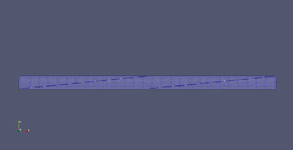
AMR mesh animation

Total Cell Count

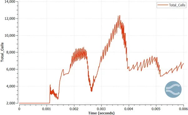
As the simulation progress the mesh refinements activates and since at the boundary the mixing and rarefaction leads to increment in total cell count as N2 dilutes at the boundary.

Change in Mean Temperature, Maximum Temperature and Pressure in the Shock-Tube

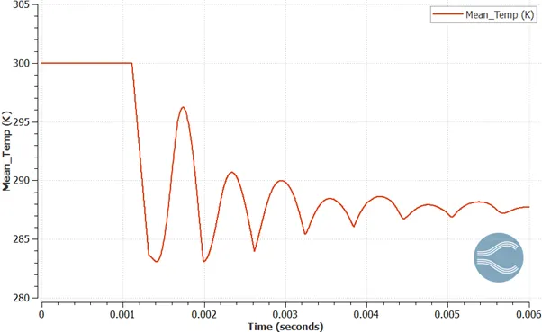
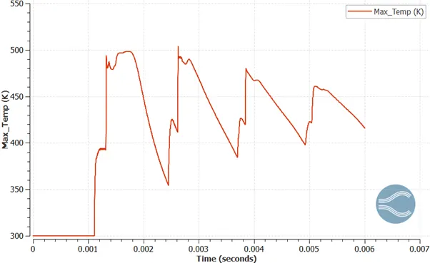
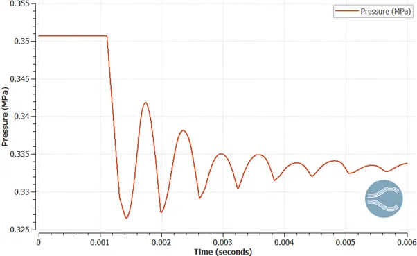
Since the shock waves travels back and forth and dampen in the process hence the mean Temp. and pressure oscillates with dampening effect to settle at a steady state.

Even though the mean temperature of the tube has fallen but the maximum temperature at certain location increases adequately.

Change in Mass fraction of N2 and velocity animation

As the shock wave bounces at the wall it hits the N2 boundary and diffuses the n2 and oscillates the boundary causing mixing effects at the boundary and such motion.

Conclusion: -

The Shock-Tube simulation is performed and analysis of the tube is done for 0.005 sec.