Week 7: Shock tube simulation project
Abstract:
A shock tube simulation is set up. Transient state analysis is carried out. Concepts like region of events, Adaptive mesh refinement is carried out. The Pressure distribution across the domain is stuidied along with other parameters like temperature and velocity.
key words: Shock tube, Converge studio, CFD , Shock wave.
Objective:
- Setting up a transient shock tube simulation
- Plottting the pressure and temperature history in the entire domain
- Plottting the cell count as a function of time.
Theory:
The shock tube is a device that is used to produce shock waves of varying strength in a controlled manner in laboratories. It has severall use foe scientific experimentation:
- High enthalpy shock tunnels to study aerothermodynamics of hypersonic flights.
- chemical shock tubes to study high temperature chemical kinetics.
- Interaction of shock waves with materials
- Blast waves and blast protection.
Tjhe initial condition of a shock tube is that it has two regions, one high pressure region called the driver section. Another low pressure region called the driven section. the driver and the driven section of the shock tube is separated by a diaphragm. When sufficient high pressure is supplied to the high pressure region, the diaphragm eventually bursts.
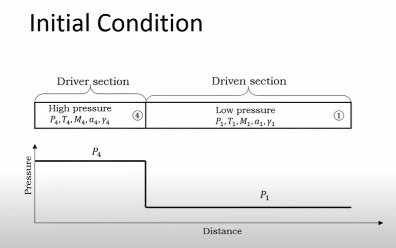
The initial profile of the pressure across the shock tube is shown above. there is a sudden jump in the pressure across the diaphragm.
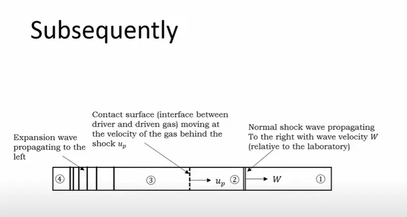
There is compressible flow within the shock tube , so the formation of shocks takes place.
As soon as the diaphragm ruptures there is a large pressure difference between the two sections . compressible flow within the tube leads to the formation of shocks. The driver section parameters are :
`p4,T4,gamma4,a4,M4` and the driven section parameters are :`p1,T1,M1,a1,gamma1`
Just behind the shock wave , there is the region of the gas . the region is marjed as 2. the shocks carry gas with them. They produce bulk motion of the gas. The shock compresses the gas from 1 to 2. so:
`(p2)/(p1),(T2)/(T1),(rho2)/(rho1)` all are more than 1.
Shocks are always supersonic, The Shock mach number may be defined as :
`Ms=W/(a1)`>1
The region 2 comprises of driven gas , that is processed by the shock waves and compressed.
In the driver section, expansion waves are present. They gradually decrease the pressure in the region. Unlike, shocks, the exoansion waves are continuos. the discontiniuty of expansion waves defies the second law of thermodynamics . Expansion process is isentropic. The section 3 has driver gas produced by the expansion waves.
A interface separates driver gas and the driven gas that is called the contact surface. It is discontinuous in nature .
There ,`P3=P2`and `u3=u2=up`
Across the contact surface the pressure remains constant.
the contact surface can be considered as piston that drives the shock wave . Across the shock, the temperature and pressure increases.
At the end there is a solid wall. the boundary condition at the solid wall is that the flow cannot penetrate the solid wall. The bulk motion of the gas on meeting the wall abruptly stops and becomes zero.
The reflected shock wave now closes in the region 2. behind the reflected wave there is the stagnant gas.
There is a significant decrease in pressure for the reflected shock wave . the region after the reflected shock wave has passed is called as the region 5.
Modelling:
Modelling the shock tube simulation inludes the geometry set up, geometry flagging, the case set up and the post procesinsg:
- Geometry:
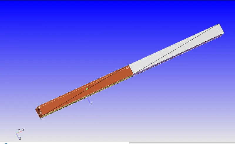
there are basically two parts in the shock tube initially. The driver section or the high pressure region and the driven section or the low pressure region.
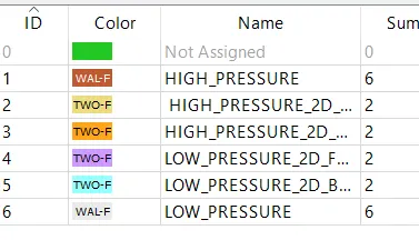
- Boundary flagging:
1) High pressure region:
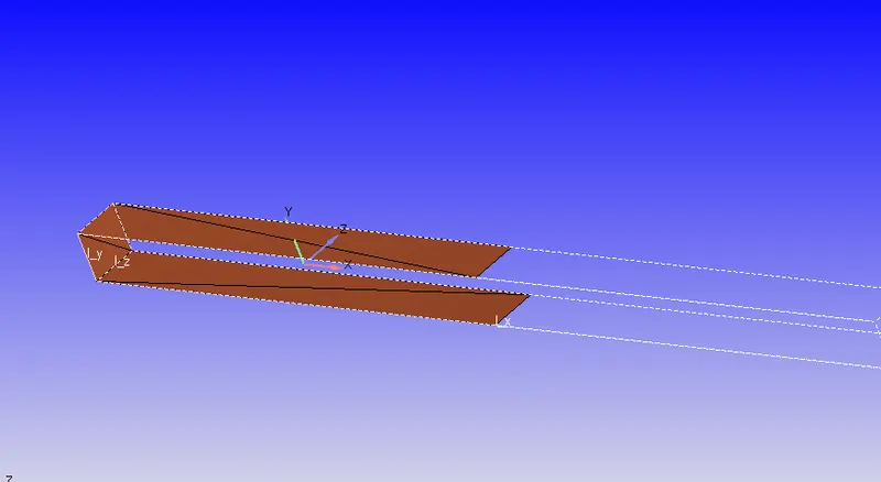
2) Low pressure region:
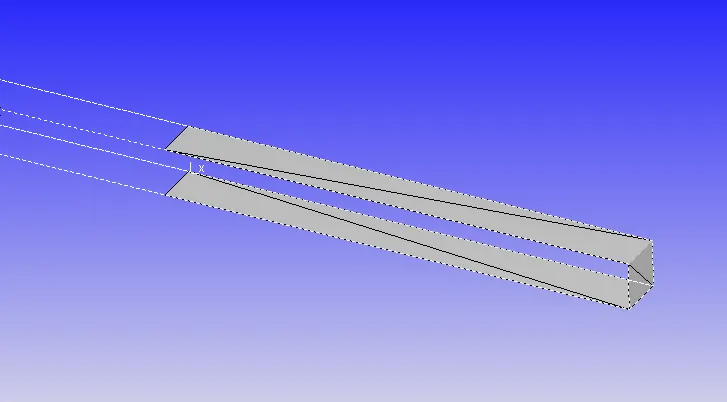
The other boundaries are the Two dimensional faces. It can be noticed here that the Converge builds a volume with the High pressure and the low pressure region.
- Case set up:
1) Application type : Time based
2) materials :
Predefined mixture : Air
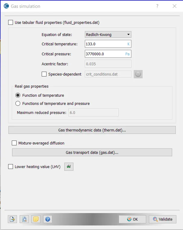
Gas simulation is checked and species is turned on.
- Gas simulation:
- Global transport parameter:
Turbulent Prandtl number : 0.9
Turbulent Schmidt number: 0.78
- Species:
O2 and N2 are dragged in as species.
3) Simulation parameters:
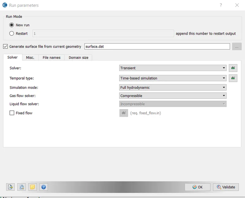
- Run parameters:
Transient simulation is ran for a Full hydrodynamic Compressible flow.
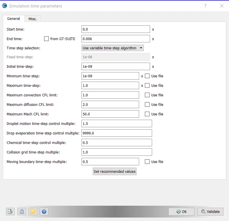
- Simulation Time parameters:
Start time : 0 seconds
End time : 0.006 seconds
Initial time step : 1e-09 seconds
Minimum time step : 1e-09 seconds
Maximum time step : 1 seconds
Maximum Cionvection CFL number : 1
Maximum Diffusion CFL number : 2
- Solver parameters:
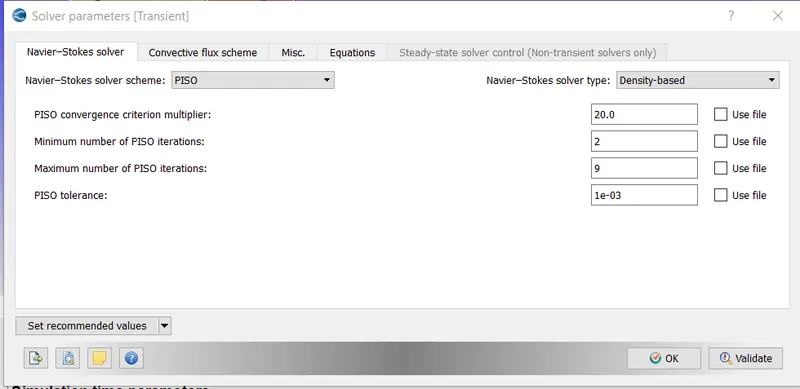
The Navier stokes solver scheme is PISO and the solver type is Density based.
Other parameters are provided by default by Converge studio.
4) Boundary Condition:
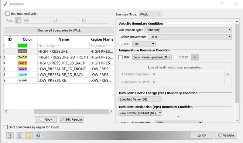
1) High pressure region:
Boundary type : Wall
Velocity Boundary conditions:
Wall motion type: Stationary
Surface movement : Fixed
Slip condition prevails
Temperature Boundary Conditions: zero Normal gradient .
2) Low pressure region:
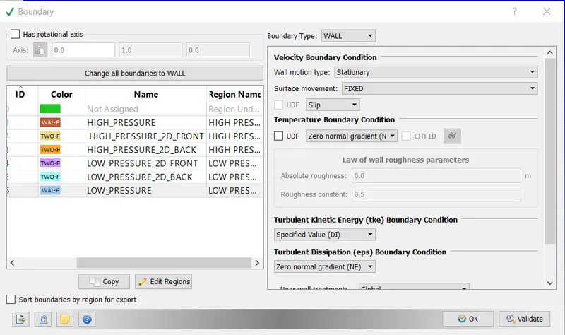
Boundary type : Wall
Velocity Boundary conditions:
Wall motion type: Stationary
Surface movement : Fixed
Slip condition prevails
Temperature Boundary Conditions: zero Normal gradient .
3) High pressure 2D : 2D boundary conditions
4) Low pressure 2D : 2D boundary conditions
5) High pressure 2D back : 2D boundary conditions
6) Low pressure 2D back: 2D boundary conditions
- Initial conditions and events:
regions and initialization :
A region is acollection of boundaries used to delinieate different areas in the geometry. Regions are useful for variety of reasons:
- Specifying initial condition by region
- Control flow between region and events
- Output results on region by region basis
- Applying grid control technique by region
There are two regions , High pressure region for the driver section and low pressure region for the driven section
High pressure region:
Pressure : 600000 pas
temperature : 300 K
species : N2 , mass fraction: 1
Low pressure region:
Pressure : 101325 Pas
Temperature: 300K
Species: O2, Mass fraction 1
Events:
With events we can connect two regions. in a simulation we cant pop the diaphragm, so with the help of events, this is done or simulated.
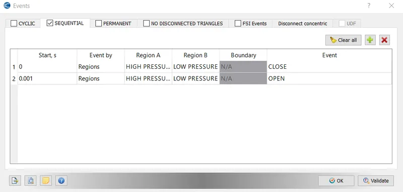
Sequential events are selected. At the beginning of the simulation, at 0 seconds the event is closed . After 1 miliseconds the event is oenned , the diaphragm pops.
- Turbulence modelling:
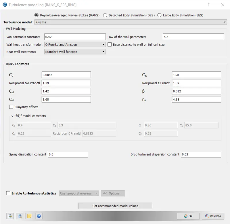
RANS is selected
turbulence model: RNG K-epsilon
the other parameters are by default provided by converge studio.
- Grid control:
Base grid :
dx=0.001,dy=0.001,dz=0.001
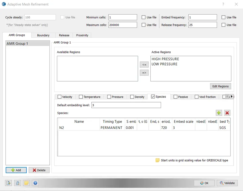
The estimated cell count without AMR is 20000
Adaptive Mesh refinemnt:
- Post processing variables:
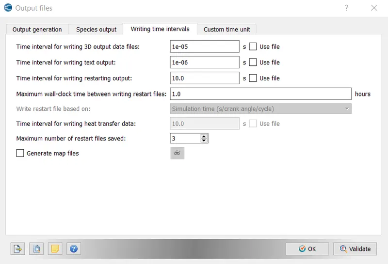
Writing time interval of the output files:
- Results and line plots:
The simulation is completed with $ processors , the command is ' mpiexec.exe -n 4 converge.exe restricted'
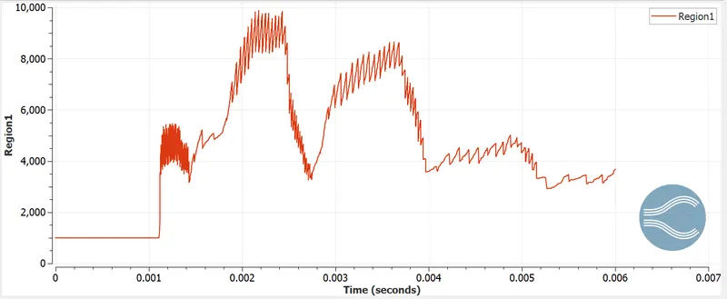
1) pressure distribution across the two regions:
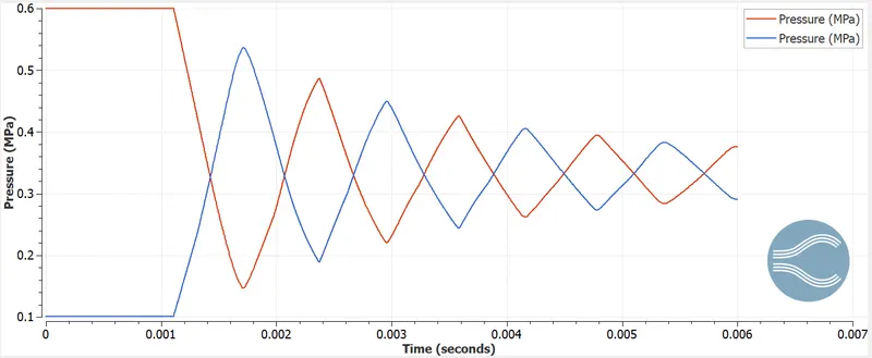
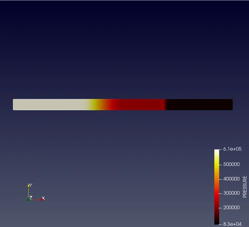
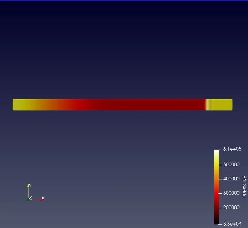
From the above plot it is seen that the pressure across the two regions the high pressure and the low pressure , remains stagnant for a 0.001 seconds. since the events are closed upto 0.001 seconds. After the events are openned , the diapgram pops, the pressure abruptly decreases for the driver section and increases for the driven section. The reflected shock wave dont have the same pressure as the original wave. The pressure decreases for the reflected wave .
2) Temperature history across the domain:
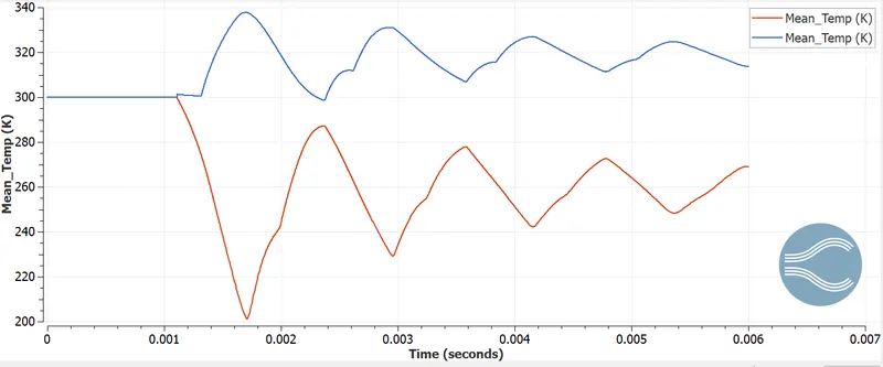
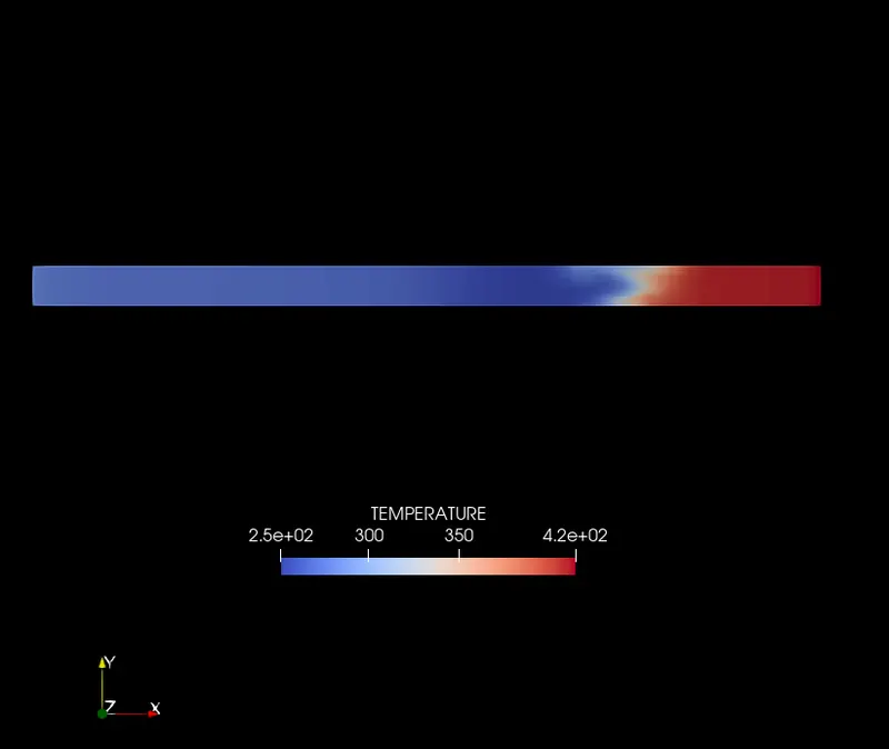
The mean temperature remains constant across the domain for the two regions till a certain time, After that it abruptly changes.
3) Cell count as a function of time:
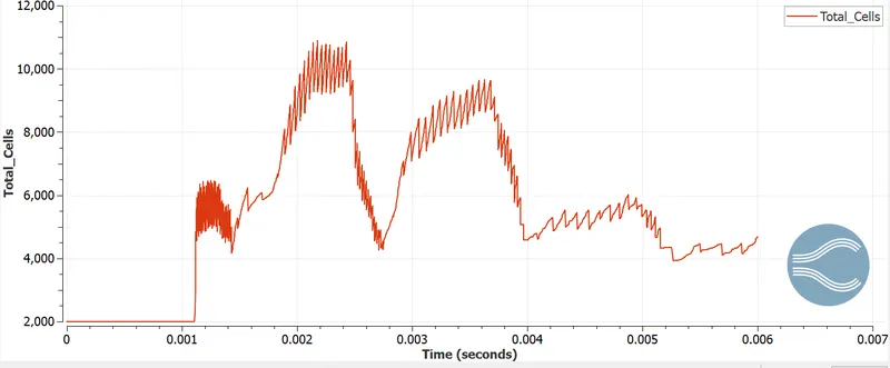
The total cell count increases abruptly, after the events are openned. The increase in cell count decreases in case of reflected waves.
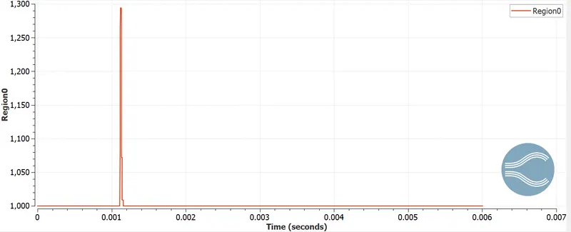
4) Cell count with time for region0:
5) cell count with time for region1:
6) Maximum Viscous CFL with time :
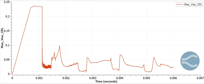
The maximum CFL is well within the limit.
Post processing in paraview:
- Mesh generation in the surface:
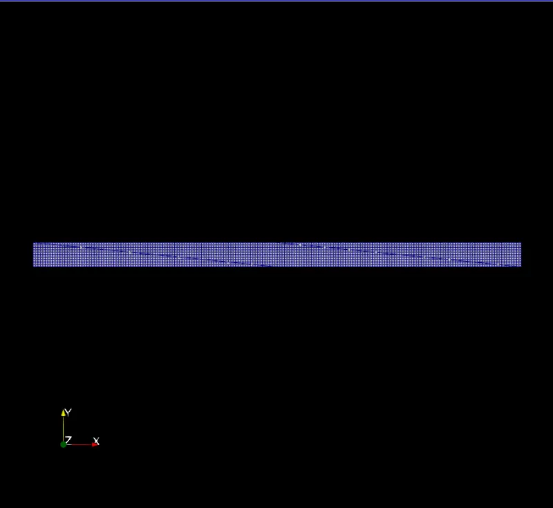
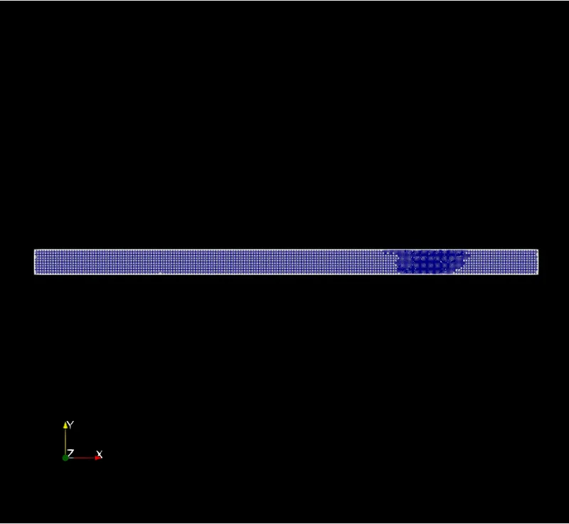
the second picture above is at the end of the time steps.
- Temperature contour:
At the end of the time steps
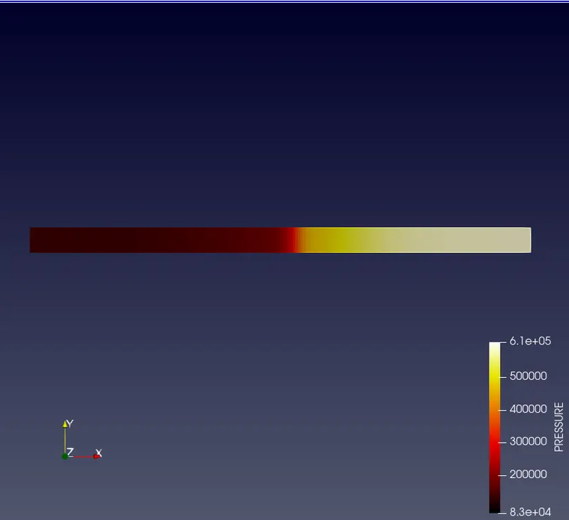
- Pressure contour:
At different time steps:
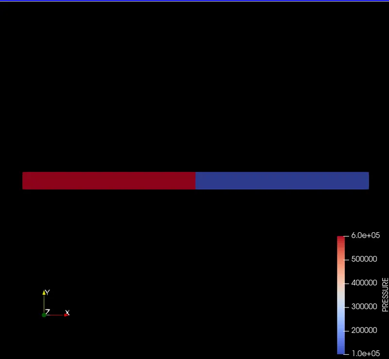
At the begining of the time step. The red part is the driver section. The blue part is the driven section. The both parts are separated by a diaphragm.
- Velocity contour:
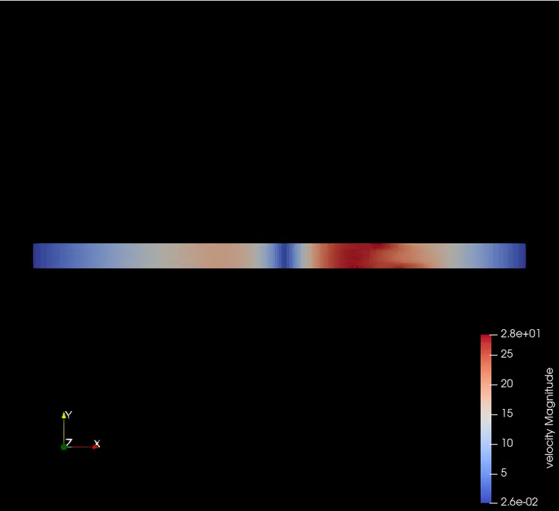
At the end of the time steps.
The animation video links are posted below:
Velocity contour animation: https://youtu.be/oElYwzdlAWA
Pressure contour animation: https://youtu.be/bA1Jjs81Ygk
Temperature contour animation: https://youtu.be/zoXhkligYzU
Conclusion:
- The shock tube modelling is set up and simulated for a transient flow
- The velocity,pressure and temperature contours are studied across the domain.