Week 7: Shock tube simulation project

Aim :-

• To setup a transient shock tube simulation.
• Plot the pressure and temperature history in the entire domain & explain the obtained result.
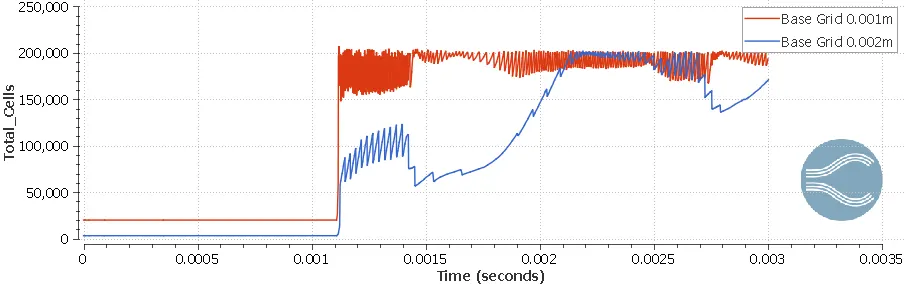
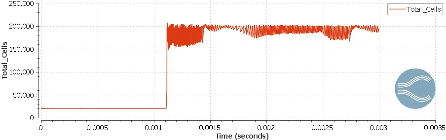
• Plot the cell count as a function of time & explain the obtained result.

Theory: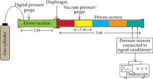

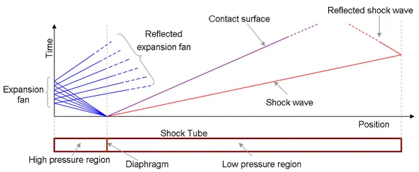
The shock tube is an instrument used to replicate and direct blast waves at a sensor or a model in order to simulate actual explosions and their effects, usually on a smaller scale. Shock tubes (and related impulse facilities such as shock tunnels, expansion tubes, and expansion tunnels) can also be used to study aerodynamic flow under a wide range of temperatures and pressures that are difficult to obtain in other types of testing facilities. Shock tubes are also used to investigate compressible flow phenomena and gas phase combustion reactions. More recently, shock tubes have been used in biomedical research to study how biological specimens are affected by blast waves.

A shock wave inside a shock tube may be generated by a small explosion (blast-driven) or by the buildup of high pressures which cause diaphragm(s) to burst and a shock wave to propagate down the shock tube (compressed-gas driven).

Generally, there are two types of Shock tubes:

Both compression-driven and blast-driven shock tubes are currently used for scientific as well as military applications. Compressed-gas driven shock tubes are more easily obtained and maintained in laboratory conditions; however, the shape of the pressure wave is different from a blast wave in some important respects and may not be suitable for some applications. Blast-driven shock tubes generate pressure waves that are more realistic to free-field blast waves. However, they require facilities and expert personnel for handling high explosives.

Working:

A simple shock tube is a tube, rectangular or circular in cross-section, usually constructed of metal, in which a gas at low pressure and a gas at high pressure are separated using some form of a diaphragm. The diaphragm suddenly bursts open under predetermined conditions to produce a wave propagating through the low pressure section. The shock that eventually forms increases the temperature and pressure of the test gas and induces a flow in the direction of the shock wave. Observations can be made in the flow behind the incident front or take advantage of the longer testing times and vastly enhanced pressures and temperatures behind the reflected wave.

The low-pressure gas, referred to as the driven gas, is subjected to the shock wave. The high-pressure gas is known as the driver gas. The corresponding sections of the tube are likewise called the driver and driven sections. The driver gas is usually chosen to have a low molecular weight, (e.g., helium or hydrogen) for safety reasons, with high speed of sound, but may be slightly diluted to 'tailor' interface conditions across the shock. To obtain the strongest shocks the pressure of the driven gas is well below atmospheric pressure (a partial vacuum is induced in the driven section before detonation).

The bursting diaphragm produces a series of pressure waves, each increasing the speed of sound behind them, so that they compress into a shock propagating through the driven gas. This shock wave increases the temperature and pressure of the driven gas and induces a flow in the direction of the shock wave but at lower velocity than the lead wave. Simultaneously, a refraction wave, often referred to as the Prandtl-Meyer wave, travels back in to the driver gas.

Applications:

Biomedical research like inserting of medicine · Military applications like missile launching · Mining purposes · Blockage removal in a Sewage plant.

Geometry:

A box of length 0.2m, with width & height of 0.01m, is modeled with 2 regions as shown.

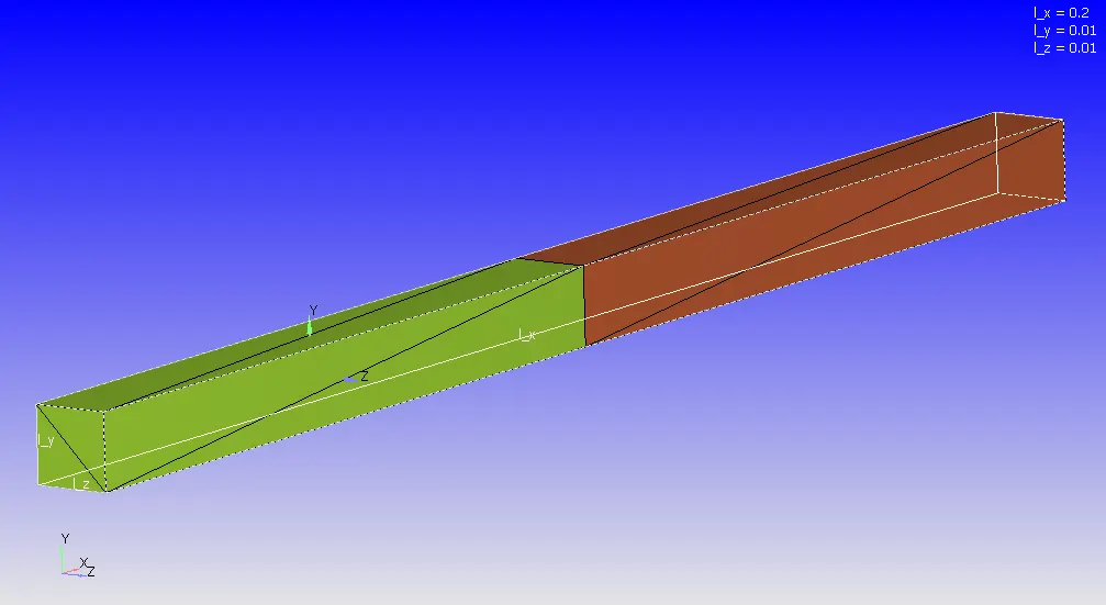
Region Green - High-Pressure Region (N2 gas)

Region Brown - Low-Pressure Region (O2 gas)

Both regions are operated by events to act as a diaphragm to obtain the shock during the simulation and to separate the regions before the explosion (i.e., the opening of the diaphragm).

CASE SETUP

1. Application Type: Time Based

2. Materials:

Predefined Mixture: Air

Gas Simulation: Default

Species:

Gas: O2 & N2

3. Solver: Transient

4. Simulation Time Parameters:

Start Time: 0 s

End Time: 0.003 s

Initial time-step: 1e-9 s

Minimum time-step: 1e-9 s

Maximum time-step: 1 s

Boundary Conditions:

High-Pressure Region ( N2, 6e5 Pa, 300K)

Low-Pressure Region ( O2, 101325 Pa, 300K)

Events:

0-0.001s (close)

0.001-0.003s (open)

Adaptive Mesh Refinement:

Base Grid 0.001m

N2 species SGS - 0.001

Mesh:

AMR is activated if the condition is satisfied.

If the condition is satisfied then,

Embedded size=(Base_Grid_Size)/2

Output:

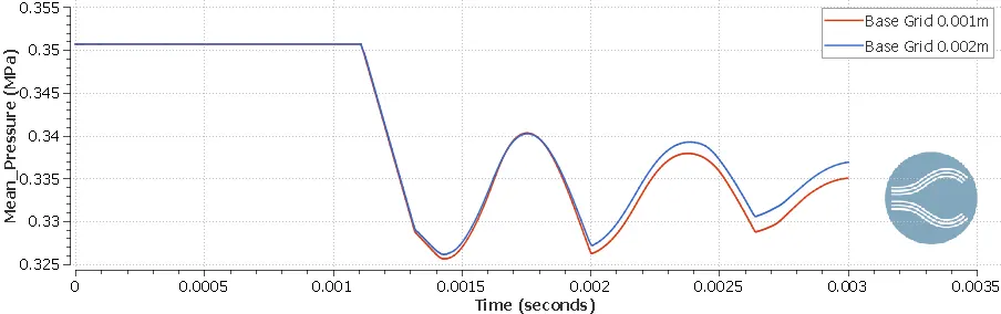
Variation of Pressure in the flow region:

Variation of Temperature in the flow region:

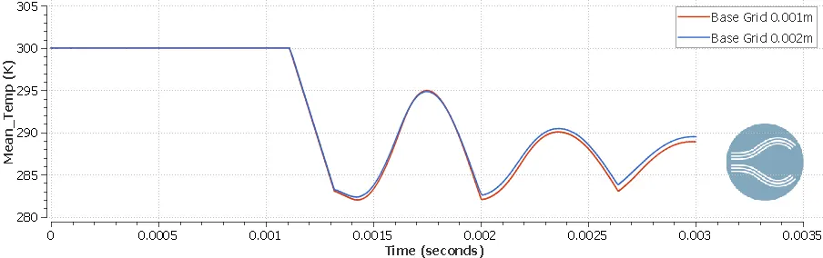
From the results obtained, base grid of 0.001 m is selected.

Steps:-

1. Upload The geometry in converge.
2. Name the boundaries, check the normal direction & flow.
3. Diagnose the geometry.
4. Region is made.
5. Simulation parameters & Boundary condition are assigned.
6. Post processing step is done.
7. All the input files are stored & executed using the command editor.
8. Data obtained after completing the simulation is post processed for graphical view.

Total Cells:

Links:-

Mass fraction & Velocity

https://drive.google.com/file/d/1_py0aLdbvyf4_wJffnv9h_c9dMsBzQQd/view?usp=share_link

Mass fraction & Pressure

https://drive.google.com/file/d/16fQPV9c3nZ2g74KCTu6ShUmEVwLDXI66/view?usp=share_link

Temperature Variation

https://drive.google.com/file/d/1FBOKg9YyrjTF9JLS8ZTjIJQNxOVO0NFv/view?usp=share_link

Density Variation

https://drive.google.com/file/d/1Cn8M5pEjDZPBcqaOI9cUkDG_B5wBuNPC/view?usp=share_link

Explanation:

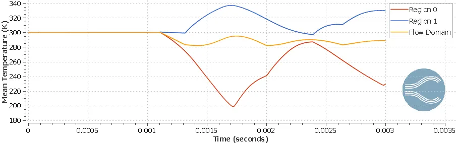
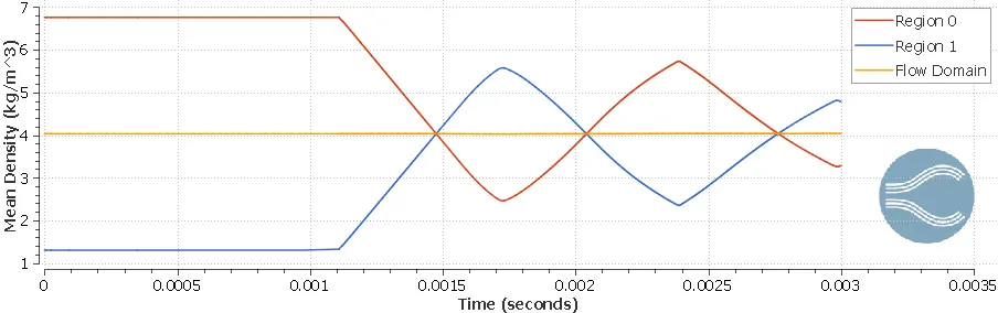
When the diaphragm is ruptured, the shock wave pushes the N2 gas towards the low-pressure region and compresses the O2 gas. But before the gases could reach the other end of the tube, the reflected shock wave pushes the N2 gas in the opposite direction thereby changing the flow direction.

There is also a sudden increase in temmp. due to shock wave in the high pressure region & the temp. is min. at low pressure region.

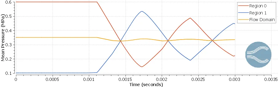
As the shock waves travels to an end of the tube , the pressure keeps decreasing until the waves get reflected back followed by sudden increase in pressure & the process continues until it reaches a steady state.

The speed of the shock wave changes its direction at zero velocity & then increases as it moves from one end to the other end.

Also the shock wave has high initial velocity which keeps decreasing with time & intensity.

Output:

Mean Temperature over Flow Time:

Mean Density over Flow Time:

Mean Pressure over Flow Time:

Conclusion:

The given setup is completed & behavior of shockwave is studied.

Further it depends on its application & condition where it is used.