Shock tube blast waves computational study using species based AMR technique.

1. AIM

Set up a transient shock tube simulation in converge, simulate it using Cygwin terminal and post-process in Paraview and check the results.

2. THEORY/EQUATIONS/FORMULAE USED

A shock tube is an instrument to produce plane propagating shockwaves by rupturing a diaphragm which separates high and low-pressure regions inside a tube. It is used to replicate and direct blast waves at a sensor or a model in order to simulate actual explosions and their effects, usually on a smaller scale. Shock tubes (and related impulse facilities such as shock tunnels, expansion tubes, and expansion tunnels) can also be used to study aerodynamic flow under a wide range of temperatures and pressures that are difficult to obtain in other types of testing facilities. Shock tubes are also used to investigate compressible flow phenomena and gas phase combustion reactions.

A shock wave inside a shock tube may be generated by a small explosion (blast-driven) or by the buildup of high pressures which cause diaphragm(s) to burst and a shock wave to propagate down the shock tube (compressed-gas driven).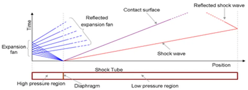

A simple shock tube is a tube, rectangular or circular in cross-section, usually constructed of metal, in which gas at low pressure and gas at high pressure is separated using some form of a diaphragm. The diaphragm suddenly bursts open under predetermined conditions to produce a wave propagating through the low-pressure section. The shock that eventually forms increases the temperature and pressure of the test gas and induces a flow in the direction of the shock wave. Observations can be made in the flow behind the incident front or take advantage of the longer testing times and vastly enhanced pressures and temperatures behind the reflected wave.

The low-pressure gas, referred to as the driven gas, is subjected to the shock wave. The high-pressure gas is known as the driver gas. The corresponding sections of the tube are likewise called the driver and driven sections. The driver gas is usually chosen to have a low molecular weight, (e.g., helium or hydrogen) for safety reasons, with a high speed of sound, but may be slightly diluted to 'tailor' interface conditions across the shock. To obtain the strongest shocks the pressure of the driven gas is well below atmospheric pressure (a partial vacuum is induced in the driven section before detonation).

The test begins with the bursting of the diaphragm. There are several methods commonly used to burst the diaphragm.

1. A mechanically-driven plunger is sometimes used to pierce it or an explosive charge may be used to burst it.
2. Use diaphragms of plastic or metals to define specific bursting pressures. Plastics are used for the lowest burst pressures, aluminum and copper for somewhat higher levels, and mild steel and stainless steel for the highest burst pressures. These diaphragms are frequently scored in a cross-shaped pattern to a calibrated depth to ensure that they rupture evenly, contouring the petals so that the full section of the tube remains open during the test time.
3. A mixture of combustible gases, with an initiator designed to produce a detonation, produces a sudden and sharp increase in what may or may not be a pressurized driver. This blast wave increases the temperature and pressure of the driven gas and induces a flow in the direction of the shock wave but at a lower velocity than the lead wave.

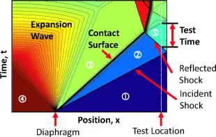
The bursting diaphragm produces a series of pressure waves, each increasing the speed of sound behind them so that they compress into a shock propagating through the driven gas. This shock wave increases the temperature and pressure of the driven gas and induces a flow in the direction of the shock wave but at a lower velocity than the lead wave. Simultaneously, a rarefaction wave, often referred to as the Prandtl-Meyer wave, travels back into the driver's gas.

The interface, across which a limited degree of mixing occurs, separates driven and driver gases is referred to as the contact surface and follow, at a lower velocity, the lead wave.

A 'Chemical Shock Tube' involves separating the driver and driven gases by a pair of diaphragms designed to fail after pre-determined delays with an end 'dump tank' of a greatly increased cross-section. This allows an extreme rapid reduction (quench) in the temperature of the heated gases.

Basic Concept

1. High-pressure driver gas expands upon diaphragm opening, creating a shock wave
2. Test gas is instantaneously compressed and heated to combustion temperatures
   by the incident and reflected shocks.
3. High-temperature experiments were monitored near the end wall.

Shock Tube Characteristics

1. Instantaneous heating/compression from shock waves.
2. Accurately known incident- and reflected-shock conditions (from incident shock MS).
3. Wide range of post-reflected shock Temperature and Pressure (600-4000 K, 0.1-1000 atm).

-------------------------------------------------------------------------------------------------------------------------

3. PROCEDURE

Case Setup

1. Geometry:- STL file is imported into Converge. The geometry for consideration is given below:

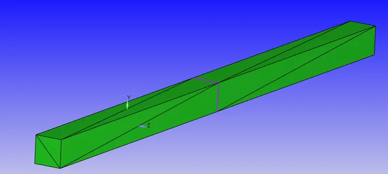
It consists of a tube which separated into two regions of different pressure. Nitrogen occupies a High-pressure region whereas oxygen occupies the low-pressure region.

2. Diagnosis:- Upon running a diagnosis check, it was noted that there were a number of Nonmanifold edge problems.

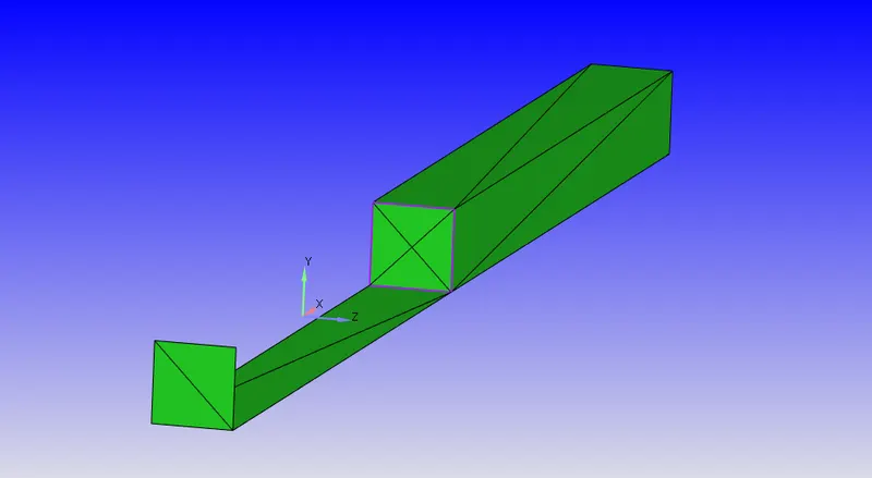
This was due to the presence of a diaphragm inside the tube. This was deleted for the purpose of this analysis. With the deletion, the problem of non-manifold edges disappeared.

3. Transform Normal:- The normals of the geometry were pointing outwards. This was transformed to ensure the normals pointed inwards.

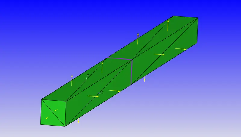
Use geometry--> transform--> Normal--> Propogate changes form sinle triangle--> Select a triangle --> Apply.

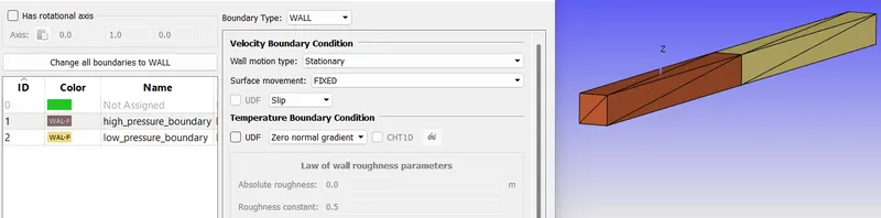
4. Boundaries:-

Both high pressure and low pressure boundaries were asigned as Slip walls.

--------------------------------------------------------------------------------------------------------------------------

Setup:

Application Type	Time-based
MATERIALS:
1. Gas simulation	Standard
2. Global Transport Parameters	Standard
3. Species	1. fluid: O2 and N2
SOLUTION PARAMETERS
Run Parameters	Transient--> Full hydrodynamic--> Compressible

--------------------------------------------------------------------------------------------------------------------------

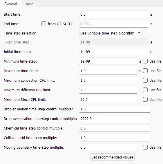
Simulation time parameters

--------------------------------------------------------------------------------------------------------------------------

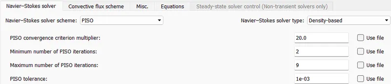
Solver parameter

Pressure Implicit Splitting Algorithm (PISO) is utilised for pressure-velocity coupling.

--------------------------------------------------------------------------------------------------------------------------

Regions and initializations

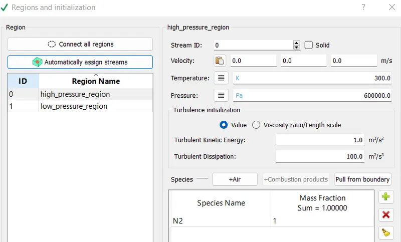
- High Pressure Region:- Pressure set to 6 bar. Mass fraction of N2 set to 1.

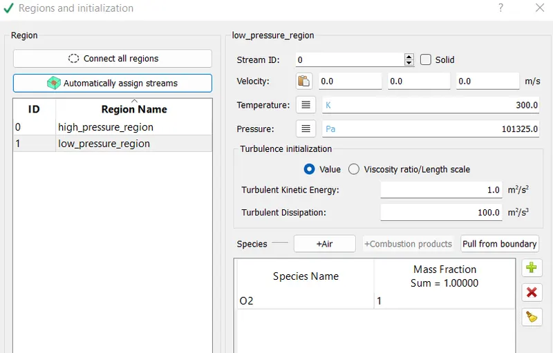
-Low Pressure Region- Pressure set to atm, Mass fraction of O2 is 1.

--------------------------------------------------------------------------------------------------------------------------

Events

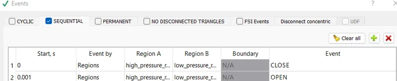
Events are used when two boundaries are in contact with each other and there is no boundary between them. the event flag creates traingles in between two regions called disconnect triangles. Here events was allocated to imitate the diaphragm rupture process. Disconntected triangles should be removed at a specific time interval.

Events can be cyclic, sequential or permanent. Traingles are crated when there is supposed to be no interaction between two regions and disconnected when there is suppossed to be an interaction.

Events are created in such a way that a diaphragm is ruptured at 0.001 seconds and the species are open to flow till the end.

--------------------------------------------------------------------------------------------------------------------------

Adaptive Mesh Refinement

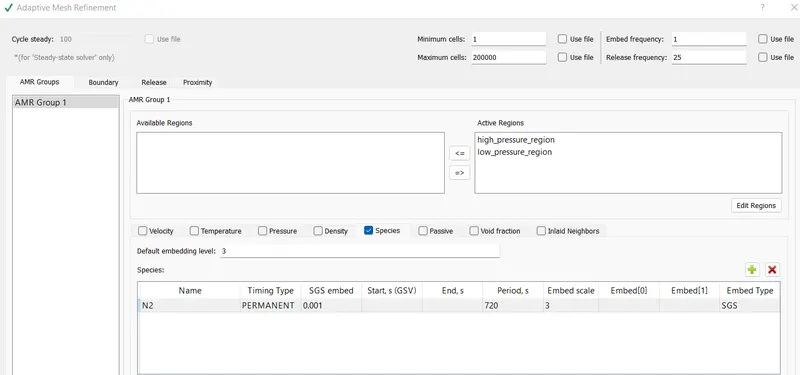
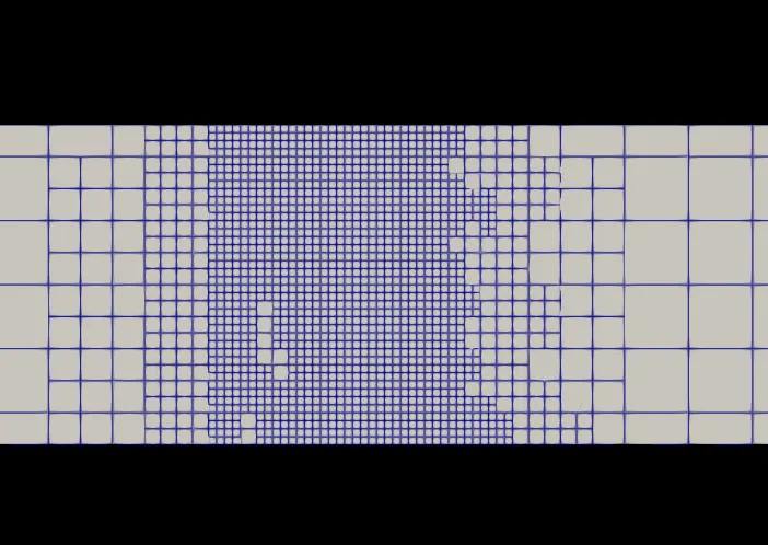
Adaptive mesh refinement feature in Converge was enabled. This was done to increase mesh resolution in the vicinity of the boundary such that cell size is sufficient to predict the boundary layer effects. AMR uses second derivative value of quantities where refinement takes place.

Here SGS embedding was set as 0.001.

--------------------------------------------------------------------------------------------------------------------------

Output Files

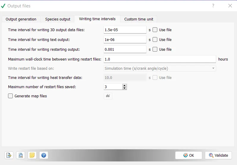
3D and text Output files writing time intervals, restart files are set as per the requirement.

--------------------------------------------------------------------------------------------------------------------------

4. POST PROCESSING RESULTS

Mesh

Initial mesh at 0th timestep.

Automatic Mesh Refinement at 20th timestep due to second derivative (curvature properties) of `N_2` concentration. Whenever solver exceeded SGS mesh was refined.

Mesh animation

----------------------------------------------------------------------------------------------------------------------------

Graphs and Contour Plots

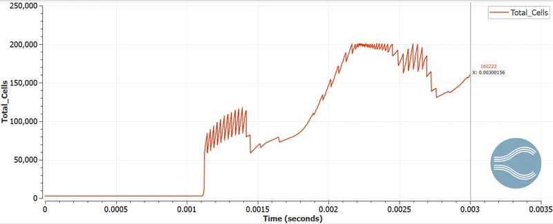
The plot shows variation of mesh size as a function of time. At 0.001sec when the diaphragm is dessimated, the event is characterized by destruction of disconnected triangles. Therefore a sudden spike with rapid fluctuations is observed. Fluctuations post t=0.001sec can be explained due to interaction of high and low pressure regions during which AMR gets activated.

Initial count of cells was observed to be 3200. As the simulation progressed maximum total cell count reached to a value of 200740 cells and approached to to 160222 at t=0.003.

-----------------------------------------------------------------------------------------------------------------------------

Pressure

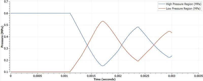
Shock wave is generated once the diaphragm is ruptured. Creation of shock wave is characterised by abrupt decrease in pressure on the high pressure side initially . The reflected waves generate a back pressure resulting in an increase in pressure on the low pressure side, which then moves on to cover the high pressure side. THere is an alternate fluctuation in pressure between regions as can be observed from the below animation as well as the plot.

Pressure Plot

Pressure Contour

Pressure Contour Animation

-----------------------------------------------------------------------------------------------------------------------------

Temperature

The temperature contour also follows the same pattern as pressure. Temperature initially decreases in N2 region initially. Reflected waves generate a backpressure causing increasing in temperature on the O2 side which then covers the high pressure side. Alternate fluctuation in Temperature can be observed in the animation as well as the line plot.

Graph

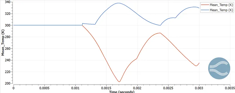
Temperature Contour

Temperature Contour Animation

-----------------------------------------------------------------------------------------------------------------------------

Velocity Contour

Similar variations can be observed in velocity profile.

Velocity Animation

-----------------------------------------------------------------------------------------------------------------------------

4. CONCLUSION

• High-Pressure N2 gas compresses the low-pressure O2 then after some compression a recirculation takes places and the low-pressure gas passes the N2.
• Pressure difference creates the shock waves are developed and it gets reflected back and forth on the walls.
• Contours also shows that the reflected shock resists the oncoming flow which in turn prevents from mixing of the two species.
• From this problem, we can understand the compressibility of gas and study the flow.
• Due to adaptive mesh refinement, the cell count is varying all the time when the expansion and contraction are taking place inside the shock tube.
• From the pressure plot, it can be concluded that after some time both the species will have common pressure as one pressure is increasing and the other is decreasing wrt time.
• The temperatures and pressures first fluctuate then may had attended the equilibrium position after some time if the simulation was run for more than 3 milliseconds.